6.2.7 Training Loop

Section Overview

This is the PyTorch workflow page where the pieces become one loop: batch, forward, loss, clear gradients, backward, update, validate, keep the best model, and predict.

Learning Goals

• Write a complete PyTorch training loop.
• Use model.train(), model.eval(), torch.no_grad(), and device transfer correctly.
• Compute average train/validation loss by sample count.
• Keep the best validation checkpoint in memory.
• Run prediction after training.

---

Look at the Loop Anatomy

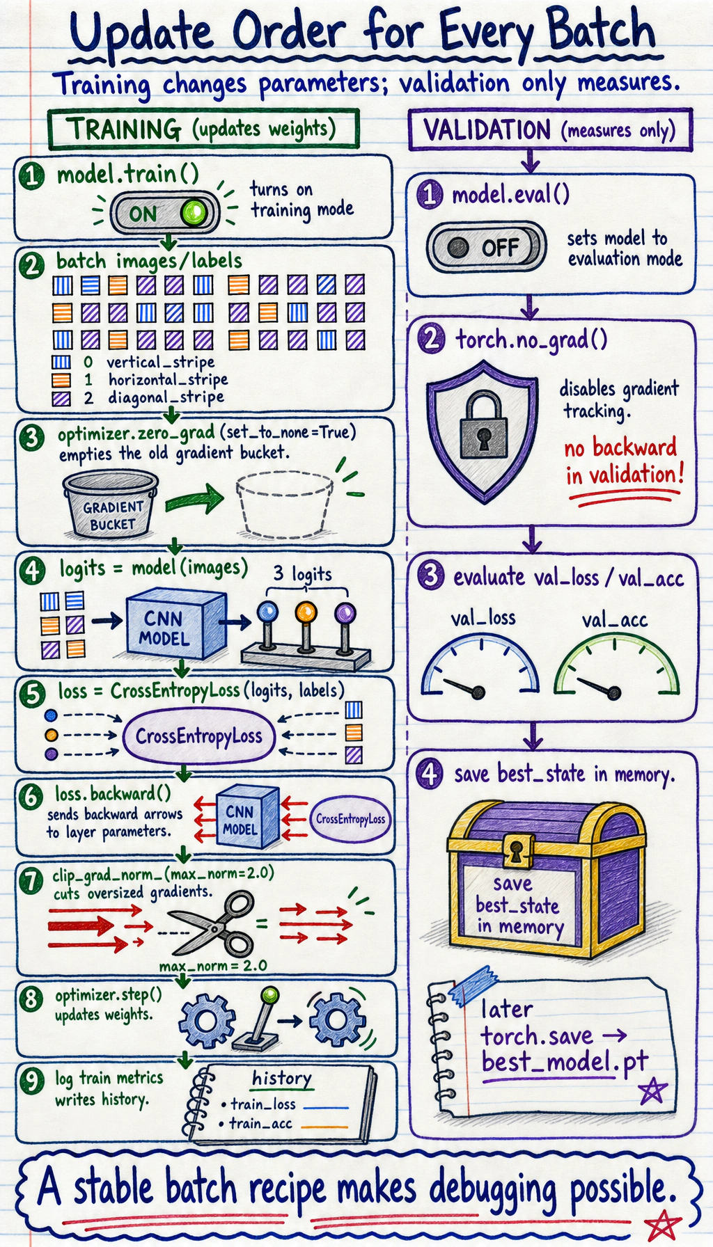
The training rhythm is:

batch→forward→loss→zero_grad→backward→optimizer.step→repeat

Validation uses a different rhythm:

eval mode→no_grad→forward→loss/metrics→no update

Why This Loop Matters

sklearn.fit() hides most of the training process. PyTorch exposes it because deep learning projects often need custom models, custom losses, custom batch logic, GPU control, logging, and checkpointing.

The same backbone appears in:

• image classification;
• text classification;
• object detection;
• fine-tuning;
• RAG reranker training;
• multimodal models.

Architecture changes, but this loop stays recognizable.

Complete Runnable Training Script

This script trains a tiny regression model on synthetic data:

y ~= 3*x1 + 2*x2 + 5

It includes device handling, train/validation split, average loss, best checkpoint, and final prediction.

import copy

import torch
from torch import nn
from torch.utils.data import DataLoader, TensorDataset, random_split

torch.manual_seed(42)

# 1. Build a small synthetic dataset
X = torch.randn(240, 2)
noise = torch.randn(240, 1) * 0.3
y = 3 * X[:, [0]] + 2 * X[:, [1]] + 5 + noise

dataset = TensorDataset(X, y)
train_dataset, val_dataset = random_split(
    dataset,
    [192, 48],
    generator=torch.Generator().manual_seed(42),
)

train_loader = DataLoader(
    train_dataset,
    batch_size=32,
    shuffle=True,
    generator=torch.Generator().manual_seed(7),
)
val_loader = DataLoader(val_dataset, batch_size=48, shuffle=False)

# 2. Select device
if torch.cuda.is_available():
    device = torch.device("cuda")
elif torch.backends.mps.is_available():
    device = torch.device("mps")
else:
    device = torch.device("cpu")


class Regressor(nn.Module):
    def __init__(self):
        super().__init__()
        self.net = nn.Sequential(
            nn.Linear(2, 16),
            nn.ReLU(),
            nn.Linear(16, 1),
        )

    def forward(self, x):
        return self.net(x)


model = Regressor().to(device)
loss_fn = nn.MSELoss()
optimizer = torch.optim.Adam(model.parameters(), lr=0.03)


def run_epoch(loader, train):
    if train:
        model.train()
    else:
        model.eval()

    total_loss = 0.0
    context = torch.enable_grad() if train else torch.no_grad()

    with context:
        for batch_x, batch_y in loader:
            batch_x = batch_x.to(device)
            batch_y = batch_y.to(device)

            pred = model(batch_x)
            loss = loss_fn(pred, batch_y)

            if train:
                optimizer.zero_grad()
                loss.backward()
                optimizer.step()

            total_loss += loss.item() * len(batch_x)

    return total_loss / len(loader.dataset)


best_val = float("inf")
best_state = None

print("training_loop_lab")
for epoch in range(1, 81):
    train_loss = run_epoch(train_loader, train=True)
    val_loss = run_epoch(val_loader, train=False)

    if val_loss < best_val:
        best_val = val_loss
        best_state = copy.deepcopy(model.state_dict())

    if epoch == 1 or epoch % 20 == 0:
        print(
            f"epoch={epoch:3d} "
            f"train_loss={train_loss:.4f} "
            f"val_loss={val_loss:.4f}"
        )

model.load_state_dict(best_state)
model.eval()

test_x = torch.tensor([[1.0, 2.0], [-1.0, 0.5], [0.0, 0.0]], device=device)
with torch.no_grad():
    preds = model(test_x).cpu()

print("best_val:", round(best_val, 4))
print("predictions:")
for row, pred in zip(test_x.cpu(), preds):
    print(f"x={row.tolist()} -> pred={pred.item():.2f}")

Expected output:

training_loop_lab
epoch=  1 train_loss=34.8472 val_loss=25.3358
epoch= 20 train_loss=0.1022 val_loss=0.0856
epoch= 40 train_loss=0.0950 val_loss=0.0776
epoch= 60 train_loss=0.0972 val_loss=0.0760
epoch= 80 train_loss=0.0936 val_loss=0.0776
best_val: 0.0734
predictions:
x=[1.0, 2.0] -> pred=12.05
x=[-1.0, 0.5] -> pred=3.00
x=[0.0, 0.0] -> pred=4.98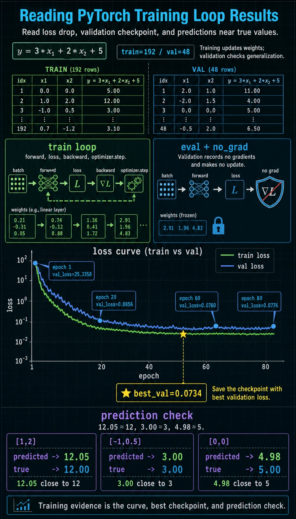

The true noiseless values are 12, 3, and 5, so the predictions are close.

How to Read the Output

Do not only check whether the script finished. Read the output as evidence:

Output	What it proves	What it does not prove
train_loss goes down	the model can fit the training data	the model generalizes
val_loss goes down	the learned pattern works on held-out samples	the split is representative of the real world
best_val is restored	the final prediction uses the best validation checkpoint	the last epoch was best
predictions near 12, 3, 5	the model learned the synthetic rule	the same model will work on messy real data

For course notes or a portfolio, keep a tiny evidence pack:

task: synthetic regression
data: 240 samples, 2 features, target ~= 3*x1 + 2*x2 + 5
best_val: 0.0734
prediction_check: [12.05, 3.00, 4.98] close to [12, 3, 5]
failure_to_try_next: increase noise to 1.0 and compare validation loss

This habit matters later. Fine-tuning, RAG evaluation, and Agent evaluation all use the same pattern: run, measure, save evidence, change one thing, compare again.

Evidence to Keep

For a training loop, the minimum evidence is not a final score. Keep the loop trace:

Device

cpu, mps, or cuda

Train Val Split

192 train samples, 48 validation samples

Loss Log

epoch 1, 20, 40, 60, 80 train_loss and val_loss

Best Checkpoint

best_val and whether best_state was restored

Prediction Probe

three test predictions compared with the noiseless targets

Debug Order

shape → dtype → device → loss → gradient → update → validation

This evidence lets someone else decide whether the model learned, overfit, failed to update, or only looked good on the last printed epoch.

Step-by-Step Breakdown

Step	Code	Why it exists
device	model.to(device), batch_x.to(device)	model and data must live on the same device
mode	model.train() / model.eval()	Dropout and BatchNorm behave differently by mode
forward	pred = model(batch_x)	current parameters make predictions
loss	loss_fn(pred, batch_y)	measure error
clear	optimizer.zero_grad()	remove old accumulated gradients
backward	loss.backward()	compute gradients
update	optimizer.step()	change parameters
validation	torch.no_grad()	evaluate without recording gradients
checkpoint	copy.deepcopy(model.state_dict())	keep the best weights, not a reference to changing weights

The copy.deepcopy detail is important. If you write best_state = model.state_dict() directly, you may keep references to tensors that continue changing.

Why Average Loss by Sample Count?

Inside each batch, loss.item() is already an average for that batch. If the last batch is smaller, a simple average of batch losses can be slightly biased.

This is why the script uses:

total_loss += loss.item() * len(batch_x)
average_loss = total_loss / len(loader.dataset)

That gives a per-sample average across the whole dataset.

Common Variations

Task	Output	Common loss
regression	[batch, 1]	nn.MSELoss() or nn.L1Loss()
multi-class classification	[batch, classes] logits	nn.CrossEntropyLoss()
binary classification	[batch, 1] logits	nn.BCEWithLogitsLoss()

For classification, track metrics in addition to loss:

• accuracy;
• precision/recall/F1 for imbalanced data;
• confusion matrix when classes are easy to confuse.

Debugging Checklist

When training behaves strangely, check in this order:

1. One batch shape: does batch_x match the first layer?
2. Label shape and dtype: does batch_y match the loss function?
3. Device: are model and data on the same device?
4. Loss value: is it finite, or nan / inf?
5. Gradients: are important parameters getting non-None gradients?
6. Updates: do parameters actually change after optimizer.step()?
7. Validation: did you use model.eval() and torch.no_grad()?

Useful probes:

print(batch_x.shape, batch_y.shape)
print(batch_x.device, next(model.parameters()).device)
print("loss:", loss.item())
for name, param in model.named_parameters():
    if param.grad is not None:
        print(name, param.grad.norm().item())
        break

Saveable Skeleton

for epoch in range(num_epochs):
    model.train()
    for batch_x, batch_y in train_loader:
        batch_x = batch_x.to(device)
        batch_y = batch_y.to(device)

        pred = model(batch_x)
        loss = loss_fn(pred, batch_y)

        optimizer.zero_grad()
        loss.backward()
        optimizer.step()

    model.eval()
    with torch.no_grad():
        for batch_x, batch_y in val_loader:
            batch_x = batch_x.to(device)
            batch_y = batch_y.to(device)
            pred = model(batch_x)
            val_loss = loss_fn(pred, batch_y)

Exercises

1. Change the optimizer from Adam to SGD(lr=0.05). How does convergence change?
2. Change hidden size from 16 to 4 and 32. Compare train and validation loss.
3. Change noise from 0.3 to 1.0. What happens to the best validation loss?
4. Add a best_epoch variable and print which epoch produced the best validation loss.
5. Convert the task to binary classification by creating labels from y > 5, then use BCEWithLogitsLoss.

Reference implementation and walkthrough

1. SGD is usually more sensitive to learning rate and may converge more slowly than Adam in this small example. If the curve is noisy, try a smaller learning rate before changing the model.
2. A hidden size of 4 may underfit, while 32 can lower training loss more easily. Prefer the setting with better validation loss, not just lower training loss.
3. More noise increases irreducible error, so the best validation loss usually becomes worse and the curve may fluctuate more.
4. Update best_epoch only when validation loss improves. The printed epoch tells you which checkpoint should be kept.
5. For binary classification, use one logit per sample or a [batch, 1] output, convert labels to float, and pass raw logits to BCEWithLogitsLoss.

Key Takeaways

• A training loop is a closed cycle: predict, measure error, compute gradients, update, validate.
• Training and validation must use different modes.
• zero_grad -> backward -> step is the core update sequence.
• Average losses by sample count when batch sizes differ.
• Keep the best checkpoint using a copied state_dict, then restore it before prediction.