3.3.9 Time Series

Section Focus

When many beginners first learn time series, the easiest misunderstanding is:

• It’s just a data column with dates added

A more reliable way to think about it is:

Once time is involved, many analyses are no longer just about “what is the value?”, but “how does it change over time?”

So the most important thing in this section is not memorizing resample() and rolling(), but first building the intuition that “time changes the way we analyze data.”

Learning Objectives

• Master creating and converting date-time types
• Learn time series indexing and slicing
• Master resampling and frequency conversion
• Learn rolling window calculations (rolling)

---

First, Build a Map

Time series is easier to understand as: “first turn dates into objects you can work with, then analyze along the time dimension”:

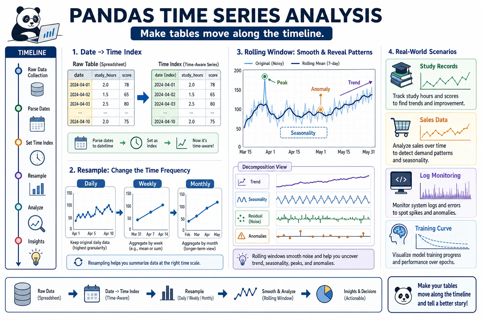
So what this section really aims to solve is:

• Why dates should not be treated like ordinary strings
• Why, once time data is organized properly, the analysis that follows becomes completely different

Why Do We Need Time Series?

Many datasets are time-related—stock prices, sales data, website traffic, service logs, model metrics… Handling time data is an essential skill in data analysis.

A More Beginner-Friendly Overall Analogy

You can think of time series as:

• Adding a real, ordered timeline to your data

With that timeline in place, you can ask not only:

• What is it now?

But also questions like:

• Is it higher or lower than last month?
• Has it been rising over the last 7 days?
• How much difference is there between the same month last year and this year?

---

Date-Time Types

Create Timestamps

import pandas as pd
import numpy as np

# Create a single timestamp
ts = pd.Timestamp("2024-01-15")
print(ts)        # 2024-01-15 00:00:00
print(ts.year)   # 2024
print(ts.month)  # 1
print(ts.day)    # 15
print(ts.day_name())  # Monday

# More formats
ts2 = pd.Timestamp("2024-01-15 14:30:00")
ts3 = pd.Timestamp(year=2024, month=3, day=20)

Convert Strings to Dates

# Convert a single column
dates = pd.Series(["2024-01-15", "2024-02-20", "2024-03-10"])
dt_series = pd.to_datetime(dates)
print(dt_series)
print(dt_series.dtype)  # datetime64[ns]

# Handle different formats
pd.to_datetime("15/01/2024", format="%d/%m/%Y")
pd.to_datetime("March 15, 2024", format="%B %d, %Y")

# Handle values that cannot be parsed
dirty = pd.Series(["2024-01-15", "not a date", "2024-03-10"])
clean = pd.to_datetime(dirty, errors="coerce")  # Unparseable values become NaT
print(clean)
# 0   2024-01-15
# 1          NaT   ← Not a Time
# 2   2024-03-10

Date Ranges

# Create a date range
dates = pd.date_range("2024-01-01", periods=10, freq="D")  # daily
print(dates)

# Different frequencies
pd.date_range("2024-01-01", periods=12, freq="ME")   # month-end
pd.date_range("2024-01-01", periods=4, freq="QE")    # quarter-end
pd.date_range("2024-01-01", "2024-12-31", freq="W")  # weekly

# Common frequency codes
# D = day, W = week, ME = month-end, MS = month-start, QE = quarter-end, YE = year-end
# h = hour, min = minute, s = second
# B = business day

What Should You Remember First When Handling Date Columns for the First Time?

The most important thing to remember first is:

A date column should preferably be converted to a real datetime type before doing any time-based analysis.

If you still keep it as a string, many things become hard to do naturally:

• Extract months
• Calculate time differences
• Do resampling

---

Time Series Data

Create a Time Series DataFrame

# Simulate daily sales data for 2024
rng = np.random.default_rng(seed=42)
dates = pd.date_range("2024-01-01", periods=365, freq="D")
sales = pd.DataFrame({
    "Date": dates,
    "Sales": rng.integers(5000, 20000, 365) + \
              np.sin(np.arange(365) * 2 * np.pi / 365) * 3000  # Add seasonality
})
sales = sales.set_index("Date")
print(sales.head())
print(sales.shape)  # (365, 1)

Extract Date Components

df = pd.DataFrame({
    "Date": pd.date_range("2024-01-01", periods=100, freq="D"),
    "Sales": rng.integers(10, 100, 100)
})

# Use the dt accessor to extract date components
df["Year"] = df["Date"].dt.year
df["Month"] = df["Date"].dt.month
df["Day"] = df["Date"].dt.day
df["Weekday"] = df["Date"].dt.day_name()
df["IsWeekend"] = df["Date"].dt.dayofweek >= 5  # 5 = Saturday, 6 = Sunday
df["WeekNumber"] = df["Date"].dt.isocalendar().week

print(df.head())

Time Index Slicing

When dates are used as the index, you can slice conveniently with strings:

# sales uses a date index
# Select data for March 2024
print(sales.loc["2024-03"])

# Select the first quarter of 2024
print(sales.loc["2024-01":"2024-03"])

# Select a specific day
print(sales.loc["2024-06-15"])

A Time Analysis Sequence That Beginners Should Remember First

A more reliable sequence is usually:

1. Convert to datetime first
2. Extract year / month / weekday first
3. Then set the date as the index
4. Finally do resampling and rolling windows

This sequence is especially important because many beginners learn in a jumpy way and end up mixing time indexes with ordinary columns.

---

Resampling (resample)

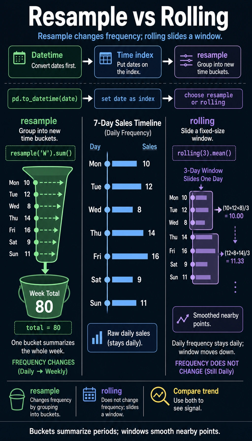
Resampling is one of the core operations in time series—it changes the time frequency of the data.

Downsampling (high frequency → low frequency)

# Daily data → monthly data
monthly = sales.resample("ME").sum()  # Aggregate by month-end
print(monthly.head())

# Daily → weekly
weekly = sales.resample("W").mean()  # Weekly average

# Daily → quarterly
quarterly = sales.resample("QE").agg({
    "Sales": ["sum", "mean", "max"]
})
print(quarterly)

Upsampling (low frequency → high frequency)

# Monthly data → daily data (needs filling)
daily = monthly.resample("D").ffill()     # Forward fill
# or
daily = monthly.resample("D").interpolate()  # Interpolation

A Beginner-Friendly Quick Reference Table

What you want to do	Better first reaction
Daily → monthly	resample() downsampling
Monthly → daily	resample() upsampling
Look at the average of the last 7 days	rolling()
Look at the average from the start up to now	expanding()

This table is especially useful for beginners because it compresses common time series operations back into a few familiar questions.

---

Rolling Window (rolling)

A rolling window calculates statistics over consecutive N data points, and it is commonly used to smooth data and calculate moving averages.

Moving Average

# 7-day moving average (smooth daily fluctuations)
sales["MA7"] = sales["Sales"].rolling(window=7).mean()

# 30-day moving average (see long-term trend)
sales["MA30"] = sales["Sales"].rolling(window=30).mean()

print(sales.head(10))
# The first 6 days of MA7 are NaN (not enough 7 days to calculate)

Other Rolling Statistics

# Rolling standard deviation (volatility)
sales["STD7"] = sales["Sales"].rolling(7).std()

# Rolling maximum
sales["MAX7"] = sales["Sales"].rolling(7).max()

# Rolling sum
sales["SUM7"] = sales["Sales"].rolling(7).sum()

expanding: Cumulative Calculations

# Cumulative mean (mean from the beginning to the current point)
sales["Cumulative Mean"] = sales["Sales"].expanding().mean()

# Cumulative maximum
sales["Historical High"] = sales["Sales"].expanding().max()

Why Is rolling So Common?

Because real time data usually fluctuates a lot. If you only look at the raw value for each day, it’s easy to get misled by the noise.

The most important value of rolling to remember first is:

• It helps you see trends through the noise

---

Calculating Time Differences

df = pd.DataFrame({
    "Signup Time": pd.to_datetime(["2023-01-15", "2023-06-20", "2024-01-10"]),
    "Last Login": pd.to_datetime(["2024-06-01", "2024-05-15", "2024-06-10"])
})

# Calculate time difference
df["Days Used"] = (df["Last Login"] - df["Signup Time"]).dt.days
print(df)

# Days since signup
df["Days Since Signup"] = (pd.Timestamp.now() - df["Signup Time"]).dt.days

---

Practice: Sales Trend Analysis

import pandas as pd
import numpy as np

rng = np.random.default_rng(seed=42)

# Create 2 years of daily sales data
dates = pd.date_range("2023-01-01", "2024-12-31", freq="D")
n = len(dates)

sales = pd.DataFrame({
    "Date": dates,
    "Sales": (
        10000 +                                    # Base value
        np.sin(np.arange(n) * 2 * np.pi / 365) * 3000 +  # Seasonality
        np.arange(n) * 5 +                         # Growth trend
        rng.normal(0, 1000, n)                     # Random fluctuation
    ).astype(int)
}).set_index("Date")

# 1. Monthly summary
monthly = sales.resample("ME").agg(
    Monthly_Sales=("Sales", "sum"),
    Daily_Average_Sales=("Sales", "mean"),
    Highest_Daily_Sales=("Sales", "max")
)
print("=== Monthly Summary ===")
print(monthly.head())

# 2. Use moving averages to see the trend
sales["MA30"] = sales["Sales"].rolling(30).mean()
print("\n=== 30-Day Moving Average (Last 5 Days) ===")
print(sales[["Sales", "MA30"]].tail())

# 3. Year-over-year growth (compare with the same month last year)
monthly_pivot = sales.resample("ME")["Sales"].sum()
monthly_pivot.index = monthly_pivot.index.to_period("M")
# Simply compare each month in 2024 vs the same month in 2023
m2024 = monthly_pivot["2024"]
m2023 = monthly_pivot["2023"]

print("\n=== 2024 vs 2023 Monthly Comparison ===")
for m24, m23 in zip(m2024.items(), m2023.items()):
    month = m24[0].month
    growth = (m24[1] - m23[1]) / m23[1] * 100
    print(f"  Month {month}: 2023={m23[1]:,.0f}, 2024={m24[1]:,.0f}, Growth={growth:+.1f}%")

# 4. Sales differences by weekday
sales_with_dow = sales.copy()
sales_with_dow["Weekday"] = sales_with_dow.index.day_name()
dow_avg = sales_with_dow.groupby("Weekday")["Sales"].mean()
print("\n=== Average Sales by Weekday ===")
print(dow_avg.sort_values(ascending=False))

What Is the Most Important Thing to Learn from This Small Practice?

The most important thing is not a specific function name, but that time analysis usually starts with these steps:

1. Summarize first
2. Then look at the trend
3. Then look at year-over-year / month-over-month changes
4. Finally look at cyclic differences

This is much more stable than jumping straight into complex forecasting.

---

Evidence to Keep

Keep this page’s proof of learning as a small evidence card:

Dataframe State

columns, dtypes, row count, missing values, and sample rows

Operation

read/write, select/filter, clean, transform, groupby, merge, or time-series step

Output

resulting table, saved file, aggregation, join result, or time index view

Failure Check

dtype mismatch, missing data, duplicated keys, chained assignment, or wrong time frequency

Expected Output

before/after table sample with the transformation reason

Summary

Operation	Method	Use
String to date	pd.to_datetime()	Type conversion
Date range	pd.date_range()	Generate consecutive dates
Extract components	.dt.year/month/day	Break down dates
Resampling	.resample()	Change time frequency
Rolling window	.rolling()	Moving average, smoothing
Cumulative calculation	.expanding()	Cumulative statistics
Time difference	subtraction + .dt.days	Calculate intervals

What Should You Take Away from This Section?

• Time series is not just “a date column added”; the analysis method changes too
• Convert dates to datetime first, then do slicing, resampling, and rolling windows
• resample changes the time frequency, while rolling helps you see local trends

---

Chapter Summary: The Big Picture of Pandas

Congratulations on completing all of the Pandas content! Let’s review:

flowchart TB
    subgraph "Chapter 2 Pandas Data Processing"
        A["2.1 Core Data Structures<br/>Series + DataFrame"] --> B["2.2 Read/Write Data<br/>CSV/Excel/JSON"]
        B --> C["2.3 Selection and Filtering<br/>loc/iloc/Boolean indexing"]
        C --> D["2.4 Data Cleaning<br/>Missing values/Duplicates/Outliers"]
        D --> E["2.5 Data Transformation<br/>apply/map/sorting/binning"]
        E --> F["2.6 Grouping and Aggregation<br/>groupby/agg/pivot_table"]
        F --> G["2.7 Data Merging<br/>merge/concat"]
        G --> H["2.8 Time Series<br/>resample/rolling"]
    end

    H --> I["✅ Pandas mastered!<br/>Ready to move on to data visualization →"]

    style I fill:#4caf50,color:#fff

✅ Self-check: Given a sales data CSV, can you use Pandas to clean missing values, group sales by month and product, and find the top-selling product for each month? Think back to the warm-up exercise from Chapter 1—isn’t it much more concise now?

---

Hands-on Exercises

Exercise 1: Date Handling

# Create a DataFrame containing dates from "2024-01-01" to "2024-12-31"
# 1. Extract month and weekday
# 2. Mark whether it is a business day
# 3. Calculate the number of business days in each month

Exercise 2: Time Series Analysis

# Use the sales data above
# 1. Calculate 7-day and 30-day moving averages
# 2. Find the months with the highest and lowest sales
# 3. Calculate month-over-month growth rates (current month vs previous month)
# 4. Analyze sales differences between weekends and weekdays

Exercise 3: Comprehensive Practice

# Simulate an app user activity dataset (365 days)
# Include: date, DAU (daily active users), new users, revenue
# 1. Calculate WAU (weekly active users) and MAU (monthly active users)
# 2. Calculate the trend of 7-day retention rate
# 3. Use rolling to calculate the 30-day average ARPU (average revenue per user)
# 4. Find the month with the fastest user growth

Reference implementation and walkthrough

• Convert date strings with pd.to_datetime first, then create calendar features such as month, weekday, quarter, and business-day flags.
• Use resample for calendar aggregation, rolling for moving windows, and pct_change for growth rates. Each method answers a different kind of question.
• For product or user metrics over time, always state the time grain. Daily, weekly, and monthly summaries can tell different stories even when they use the same raw events.