3.5.3 SQL Basics

Section Overview

When many beginners first learn SQL, what trips them up most is not that the syntax is too much, but that they don’t know:

• What the relationship is between SQL and Pandas
• How the query order should be organized in their head

So the most important thing in this section is not memorizing every syntax rule first, but building a judgment:

In essence, SQL is a stable language for asking tables questions.

Learning Objectives

• Master the four basic SQL operations: create, read, update, delete
• Use SELECT queries fluently
• Learn WHERE condition filtering
• Master JOIN for combining multiple tables
• Understand GROUP BY for grouped aggregation

---

First, Build a Map

The best way for beginners to understand SQL is not to “memorize the syntax book from start to finish,” but to first see clearly:

flowchart LR
    A["SELECT what to choose"] --> B["FROM which table"]
    B --> C["WHERE what to filter first"]
    C --> D["GROUP BY how to group"]
    D --> E["ORDER BY how to sort last"]

So what this section really wants to solve is:

• How SQL queries actually flow in your head
• Why it corresponds to Pandas filtering, grouping, and merging

What Is SQL?

SQL (Structured Query Language) is the language used to “talk” to databases. Whether you use SQLite, MySQL, or PostgreSQL, the SQL syntax is basically the same.

flowchart LR
    A["You (human)"] -->|"Write SQL"| B["Database engine"]
    B -->|"Return results"| A

    style A fill:#e3f2fd,stroke:#1565c0,color:#333
    style B fill:#e8f5e9,stroke:#2e7d32,color:#333

The Relationship Between SQL and Pandas

What SQL can do, Pandas can do for the most part too. In fact, many Pandas method names, such as merge and groupby, were borrowed from SQL. Learning them side by side works better.

A Better Analogy for Beginners

You can think of SQL as:

• You asking the database questions

And these questions are usually very straightforward:

• Which columns do I want?
• Which rows do I want?
• How should I group them?
• How do I connect two tables?

This analogy is especially useful for beginners because it pulls SQL back from “another language” into “how do I ask the table questions?”

---

Preparation: Create a Practice Database

All examples in this section are based on this practice database. Please run the following first:

import sqlite3

conn = sqlite3.connect(":memory:")  # In-memory database, disappears when closed
cursor = conn.cursor()

# Create users table
cursor.execute("""
    CREATE TABLE users (
        id INTEGER PRIMARY KEY,
        name TEXT NOT NULL,
        age INTEGER,
        city TEXT,
        salary REAL
    )
""")

# Create orders table
cursor.execute("""
    CREATE TABLE orders (
        order_id INTEGER PRIMARY KEY,
        user_id INTEGER,
        product TEXT,
        amount REAL,
        order_date TEXT,
        FOREIGN KEY (user_id) REFERENCES users(id)
    )
""")

# Insert user data
users_data = [
    (1, "Alice", 28, "Beijing", 15000),
    (2, "Bob", 35, "Shanghai", 22000),
    (3, "Charlie", 22, "Guangzhou", 8000),
    (4, "Diana", 42, "Beijing", 35000),
    (5, "Ethan", 30, "Shanghai", 18000),
    (6, "Fiona", 26, "Shenzhen", 12000),
]
cursor.executemany("INSERT INTO users VALUES (?, ?, ?, ?, ?)", users_data)

# Insert order data
orders_data = [
    (101, 1, "iPhone", 7999, "2024-11-01"),
    (102, 1, "AirPods", 999, "2024-11-05"),
    (103, 2, "MacBook", 14999, "2024-11-10"),
    (104, 3, "iPad", 3999, "2024-11-15"),
    (105, 2, "Keyboard", 599, "2024-11-20"),
    (106, 4, "Monitor", 2999, "2024-12-01"),
    (107, 5, "Mouse", 299, "2024-12-05"),
]
cursor.executemany("INSERT INTO orders VALUES (?, ?, ?, ?, ?)", orders_data)

conn.commit()

# Define a helper function for easier querying
def query(sql):
    cursor.execute(sql)
    cols = [desc[0] for desc in cursor.description]
    rows = cursor.fetchall()
    # Print header
    print(" | ".join(cols))
    print("-" * (len(" | ".join(cols))))
    for row in rows:
        print(" | ".join(str(v) for v in row))
    print()

---

Query Data (SELECT)

SELECT is the most commonly used SQL statement. It is used to retrieve data from tables.

Basic Queries

-- Query all columns
SELECT * FROM users;

-- Query specific columns
SELECT name, age, city FROM users;

-- Give columns aliases
SELECT name AS name, age AS age FROM users;

query("SELECT * FROM users")
# id | name | age | city | salary
# 1 | Alice | 28 | Beijing | 15000
# 2 | Bob | 35 | Shanghai | 22000
# ...

DISTINCT: Remove Duplicates

-- Query all unique cities
SELECT DISTINCT city FROM users;

LIMIT: Limit the Number of Rows

-- Take only the first 3 rows
SELECT * FROM users LIMIT 3;

The Safest Default Order When Writing Your First Query

A more reliable order is usually:

1. Write SELECT first
2. Then write FROM
3. Then decide whether to add WHERE
4. Finally add sorting and grouping

This is less confusing than trying to mix all clauses together right away.

---

Condition Filtering (WHERE)

WHERE is like Pandas boolean indexing and is used to filter rows that meet certain conditions.

Basic Comparisons

-- Age greater than 30
SELECT * FROM users WHERE age > 30;

-- City is Beijing
SELECT * FROM users WHERE city = 'Beijing';

-- Salary between 10000 and 20000
SELECT * FROM users WHERE salary BETWEEN 10000 AND 20000;

Combined Conditions

-- AND: both conditions must be true
SELECT * FROM users WHERE city = 'Beijing' AND age > 25;

-- OR: either condition
SELECT * FROM users WHERE city = 'Beijing' OR city = 'Shanghai';

-- IN: within a list
SELECT * FROM users WHERE city IN ('Beijing', 'Shanghai', 'Shenzhen');

-- NOT: negation
SELECT * FROM users WHERE city NOT IN ('Beijing');

Pattern Matching (LIKE)

-- % matches any characters (similar to Pandas str.contains)
SELECT * FROM users WHERE name LIKE 'A%';    -- starts with "A"
SELECT * FROM users WHERE name LIKE '%e';    -- ends with "e"
SELECT * FROM users WHERE email LIKE '%@mail%'; -- contains "@mail"

Handling NULL

-- Check whether it is empty (do not use = NULL)
SELECT * FROM users WHERE city IS NULL;
SELECT * FROM users WHERE city IS NOT NULL;

SQL vs Pandas Comparison

Requirement	SQL	Pandas
Age greater than 30	WHERE age > 30	df[df["age"] > 30]
City is Beijing	WHERE city = 'Beijing'	df[df["city"] == "Beijing"]
Multiple conditions with AND	WHERE age > 30 AND city = 'Beijing'	df[(df["age"] > 30) & (df["city"] == "Beijing")]
Multiple conditions with OR	WHERE city IN ('Beijing', 'Shanghai')	df[df["city"].isin(["Beijing", "Shanghai"])]
Pattern matching	WHERE name LIKE 'A%'	df[df["name"].str.startswith("A")]
Empty values	WHERE city IS NULL	df[df["city"].isna()]

A Comparison Table Beginners Should Remember First

Question in your head	More like which SQL clause
Only look at records that meet the condition	WHERE
See which unique values exist in a table	DISTINCT
Just take the first few rows to check	LIMIT
Connect two tables	JOIN
Group first, then aggregate	GROUP BY

This table is especially useful for beginners because it compresses SQL back into a few common types of questions instead of a long list of keywords.

---

Sorting (ORDER BY)

-- Sort by salary ascending (default)
SELECT * FROM users ORDER BY salary;

-- Sort by salary descending
SELECT * FROM users ORDER BY salary DESC;

-- Sort by city first, then salary descending within the same city
SELECT * FROM users ORDER BY city, salary DESC;

Why Is ORDER BY Often Written Last?

Because sorting is more like:

• The result is already there, and now I want to see it in a certain order

This is not the same kind of problem as:

• Filtering first
• Grouping first

---

Aggregate Functions and Grouping (GROUP BY)

Common Aggregate Functions

Function	Purpose	Example
COUNT(*)	Count rows	How many records in total
SUM(col)	Sum values	Total salary
AVG(col)	Average value	Average age
MAX(col)	Maximum value	Highest salary
MIN(col)	Minimum value	Lowest age

-- Basic aggregation
SELECT COUNT(*) AS total_people, AVG(salary) AS avg_salary, MAX(salary) AS highest_salary
FROM users;

GROUP BY: Grouped Statistics

-- Count people and average salary by city
SELECT city, COUNT(*) AS people_count, AVG(salary) AS avg_salary
FROM users
GROUP BY city;

city | people_count | avg_salary
Beijing | 2 | 25000.0
Shanghai | 2 | 20000.0
Guangzhou | 1 | 8000.0
Shenzhen | 1 | 12000.0

HAVING: Filter Grouped Results

-- Find cities with average salary above 15000
SELECT city, AVG(salary) AS avg_salary
FROM users
GROUP BY city
HAVING avg_salary > 15000;

WHERE vs HAVING

• WHERE filters before grouping (filters raw rows)
• HAVING filters after grouping (filters aggregated results)

SQL Execution Order

The writing order of SQL is different from the execution order:

flowchart TD
    A["1. FROM<br/>Determine data source"] --> B["2. WHERE<br/>Filter raw rows"]
    B --> C["3. GROUP BY<br/>Group"]
    C --> D["4. HAVING<br/>Filter groups"]
    D --> E["5. SELECT<br/>Choose columns"]
    E --> F["6. ORDER BY<br/>Sort"]
    F --> G["7. LIMIT<br/>Limit rows"]

    style A fill:#e3f2fd,stroke:#1565c0,color:#333
    style E fill:#fff3e0,stroke:#e65100,color:#333

---

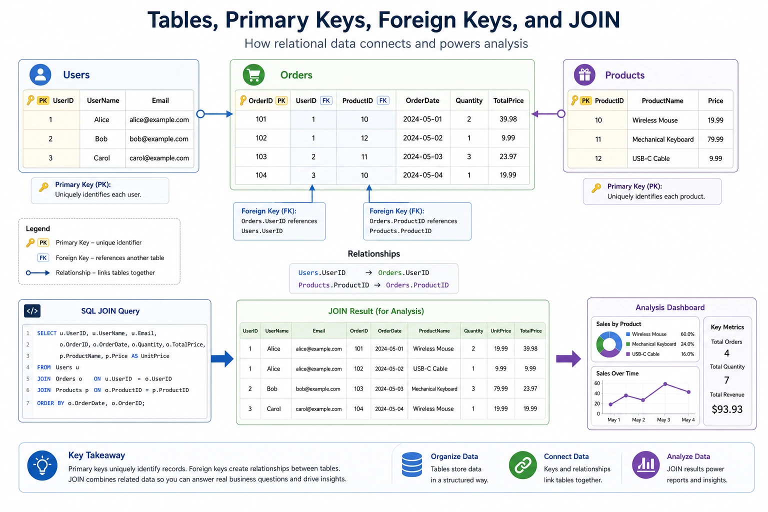
Joining Multiple Tables (JOIN)

JOIN is one of SQL’s most powerful features. It lets you combine data from multiple tables.

INNER JOIN

Returns only rows that match in both tables.

-- Query each user's order information
SELECT users.name, orders.product, orders.amount
FROM users
INNER JOIN orders ON users.id = orders.user_id;

name	product	amount
Zhang San	iPhone	7999.0
Zhang San	AirPods	999.0
Li Si	MacBook	14999.0
Wang Wu	iPad	3999.0
Li Si	Keyboard	599.0
Zhao Liu	Monitor	2999.0
Qian Qi	Mouse	299.0

Note: Sun Ba has no orders, so he does not appear in the result.

LEFT JOIN

Returns all rows from the left table; unmatched rows from the right table are shown as NULL.

-- Query all users and their orders (including users with no orders)
SELECT users.name, orders.product, orders.amount
FROM users
LEFT JOIN orders ON users.id = orders.user_id;

name | product | amount
Zhang San | iPhone | 7999.0
Zhang San | AirPods | 999.0
Li Si | MacBook | 14999.0
...
Sun Ba | None | None       ← No orders, but still shown

Comparison of JOIN Types

flowchart TD
    A["JOIN types"] --> B["INNER JOIN<br/>Only rows that exist on both sides"]
    A --> C["LEFT JOIN<br/>Keep all left rows, fill missing right values with NULL"]
    A --> D["RIGHT JOIN<br/>Keep all right rows, fill missing left values with NULL"]
    A --> E["FULL OUTER JOIN<br/>Keep all rows from both sides"]

    style B fill:#e8f5e9,stroke:#2e7d32,color:#333
    style C fill:#e3f2fd,stroke:#1565c0,color:#333
    style D fill:#fff3e0,stroke:#e65100,color:#333
    style E fill:#f3e5f5,stroke:#7b1fa2,color:#333

SQL JOIN vs Pandas merge

SQL	Pandas
INNER JOIN	pd.merge(how="inner")
LEFT JOIN	pd.merge(how="left")
RIGHT JOIN	pd.merge(how="right")
ON users.id = orders.user_id	on="user_id" or left_on=, right_on=

Practical Combination: JOIN + GROUP BY

-- Query each user's total order amount
SELECT users.name, COUNT(orders.order_id) AS order_count, SUM(orders.amount) AS total_spent
FROM users
LEFT JOIN orders ON users.id = orders.user_id
GROUP BY users.id, users.name
ORDER BY total_spent DESC;

---

Insert, Update, Delete (INSERT / UPDATE / DELETE)

Insert Data

-- Insert one row
INSERT INTO users (name, age, city, salary) VALUES ('Zhou Jiu', 29, 'Hangzhou', 16000);

-- Insert multiple rows
INSERT INTO users (name, age, city, salary) VALUES
    ('Wu Shi', 33, 'Chengdu', 13000),
    ('Zheng Shiyi', 27, 'Nanjing', 11000);

Update Data

-- Give Zhang San a raise
UPDATE users SET salary = 18000 WHERE name = 'Zhang San';

-- Give all Beijing employees a 10% raise
UPDATE users SET salary = salary * 1.1 WHERE city = 'Beijing';

Always Add WHERE for UPDATE!

UPDATE users SET salary = 0; will set the salary of all users to zero! Forgetting WHERE is one of the most common disasters in database operations.

Delete Data

-- Delete a specific record
DELETE FROM users WHERE name = 'Zhou Jiu';

-- Delete all records with age less than 20
DELETE FROM users WHERE age < 20;

Always Add WHERE for DELETE!

DELETE FROM users; will delete all data in the table! Think carefully before doing this.

The Safest Default Order When Learning SQL for the First Time

A more reliable order is usually:

1. First write SELECT / FROM / WHERE correctly
2. Then add ORDER BY
3. Then add GROUP BY / HAVING
4. Finally learn JOIN and insert, update, delete

This is less confusing than memorizing all syntax blocks at once.

---

SQL Statement Quick Reference

Operation	SQL Syntax	Description
Query all	SELECT * FROM table_name	Get all data
Query specific columns	SELECT col1, col2 FROM table_name	Get some columns
Condition filtering	SELECT ... WHERE condition	Filter rows
Sorting	ORDER BY col DESC	Sort descending
Limit rows	LIMIT 10	Take the first N rows
Remove duplicates	SELECT DISTINCT col	Unique values
Aggregation	COUNT / SUM / AVG / MAX / MIN	Statistical calculations
Grouping	GROUP BY col	Grouped statistics
Group filtering	HAVING condition	Filter grouped results
Inner join	INNER JOIN table ON condition	Intersection of two tables
Left join	LEFT JOIN table ON condition	All rows from the left table
Insert	INSERT INTO table VALUES (...)	Add data
Update	UPDATE table SET col=value WHERE condition	Modify data
Delete	DELETE FROM table WHERE condition	Delete data

---

Evidence to Keep

Keep this page’s proof of learning as a small evidence card:

Schema

table names, keys, relationships, and sample rows

Query

SQL or Python database code used

Output

result rows, row count, or saved extract

Failure Check

wrong join key, unsafe query, missing transaction, or schema mismatch

Expected Output

query plus result table and one data-quality note

Summary

SQL is the language for “talking” to databases. Its core consists of four types of operations:

Category	Keyword	Purpose
Read	SELECT	Query data (most common)
Create	INSERT	Insert new data
Update	UPDATE	Modify existing data
Delete	DELETE	Remove data

Among them, SELECT together with WHERE, JOIN, and GROUP BY can cover most data analysis tasks.

What You Should Take Away From This Section

• The most important thing about SQL is not that it has many keywords, but whether you can use it steadily to ask tables questions
• If you first think, “Which columns do I want, which rows do I want, and how should I group them?”, writing SQL will be much more stable than memorizing syntax
• Once WHERE / GROUP BY / JOIN becomes clear, most later queries can be understood step by step

---

Hands-On Exercises

Exercise 1: Basic Queries

-- Using the practice database above, complete the following queries:
-- 1. Query all users in Shanghai
-- 2. Query the top 3 people with the highest salaries
-- 3. Query the average salary for each city, sorted by average salary in descending order

Exercise 2: JOIN Queries

-- 1. Query the names of all users and the products they have bought
-- 2. Query users who have never placed an order
--    Hint: LEFT JOIN + WHERE orders.order_id IS NULL
-- 3. Query the total order amount for each user, including users with no orders (show as 0)

Exercise 3: Comprehensive Analysis

-- Complete this with one SQL statement:
-- Query the user name, number of orders, and total spending for users whose total spending exceeds 5000
-- Sort by total spending in descending order

Reference implementation and walkthrough

• Filtering exercises should use WHERE, sorting and top-k should use ORDER BY ... LIMIT, and city averages should use GROUP BY city with AVG(...).
• For order reports, use JOIN when only customers with orders matter and LEFT JOIN when customers without orders must stay visible. COALESCE is useful for showing zero instead of null total spend.
• For summary filters such as total spend greater than a threshold, aggregate first and use HAVING, not WHERE, because the condition depends on grouped results.