3.3.6 Data Transformation

Section Overview

Many beginners start to feel a bit confused when they get here:

• apply
• map
• replace
• rank
• cut

You may know all these names, but once they show up in a problem, it’s easy to mix up which one to use first.

So the most important thing in this section is not memorizing more functions, but first building a clear judgment:

Am I trying to “change values”, “create a new column”, “do sorting/ranking”, or “split continuous values into bins”?

Learning Objectives

• Understand how apply, map, and applymap work and how they differ
• Learn sorting (sort_values) and ranking (rank)
• Master data replacement and mapping

---

Build a mental map first

Data transformation is easier to understand by asking: “What do I want this column to become?”

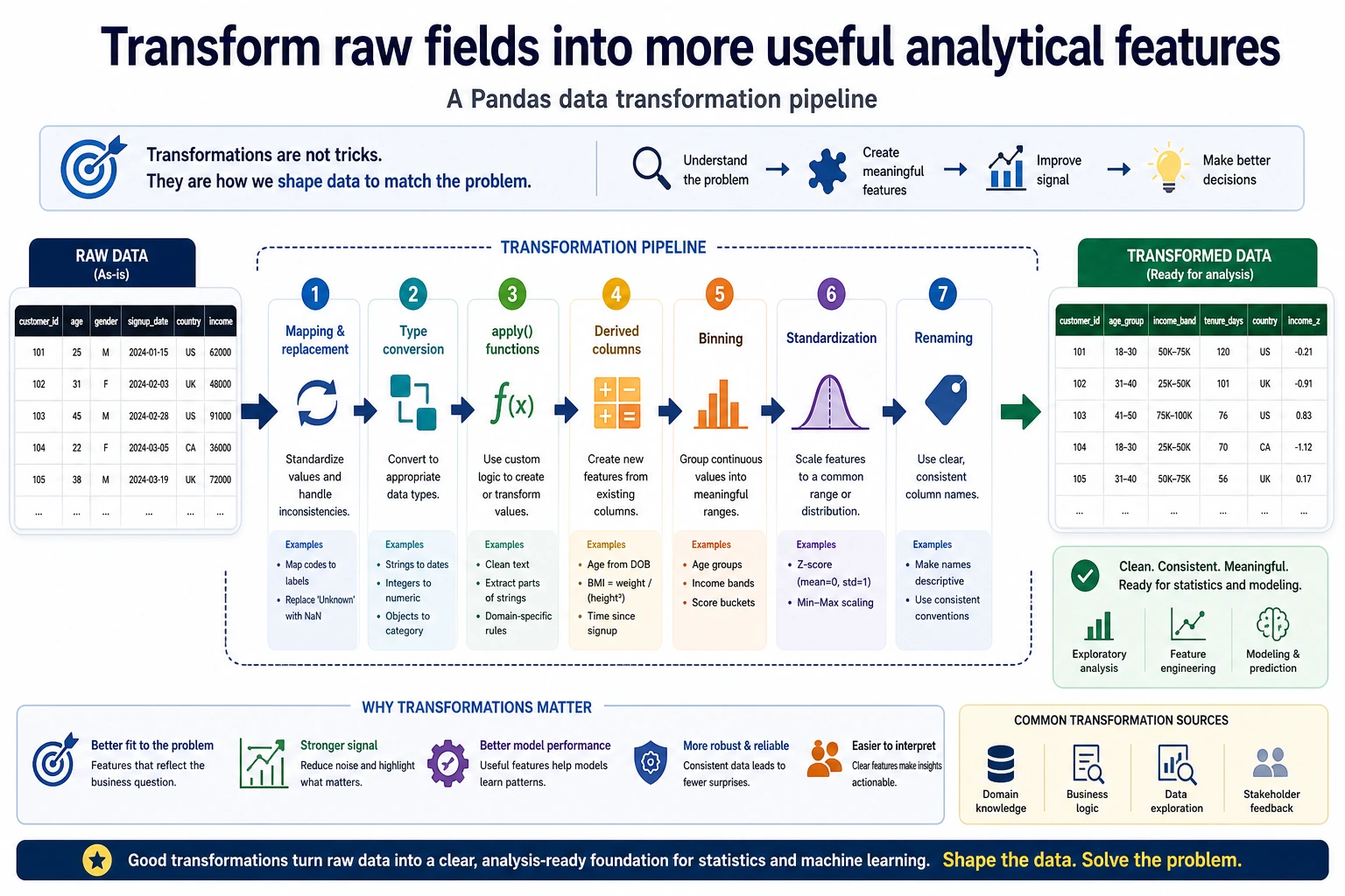
So what this section really aims to solve is:

• What each transformation action is used for
• When to think of map first, and when to think of apply first

apply: Apply a function to rows or columns

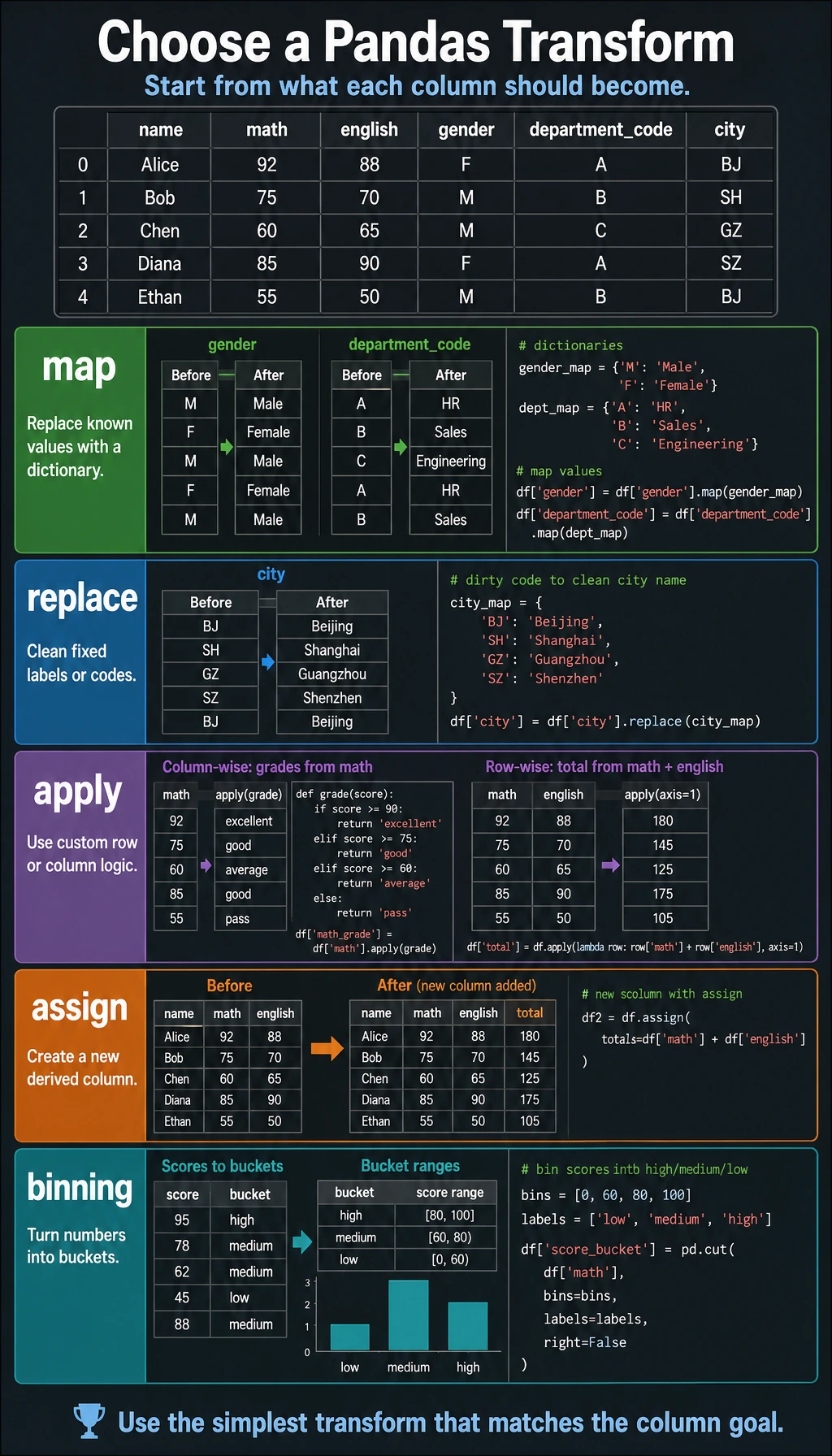
apply is one of Pandas’ most flexible transformation tools — it can apply any function to each row or each column.

A better beginner-friendly analogy

You can think of data transformation as:

• “translating, processing, and relabeling” raw data

Sometimes you just want to:

• translate codes into English

Sometimes you want to:

• calculate a new result from several columns in one row

Sometimes you want to:

• split continuous numbers into three levels: high, medium, and low

All of these look like “transformations,” but they are actually different types of problems.

Apply to a column (Series)

import pandas as pd
import numpy as np

df = pd.DataFrame({
    "name": ["Zhang San", "Li Si", "Wang Wu", "Zhao Liu"],
    "math": [85, 92, 78, 95],
    "english": [90, 88, 72, 85]
})

# Apply a built-in function to a single column
print(df["math"].apply(np.sqrt))  # square root of each score

# Apply a custom function to a single column
def grade(score):
    if score >= 90: return "excellent"
    elif score >= 80: return "good"
    elif score >= 70: return "average"
    else: return "pass"

df["math_grade"] = df["math"].apply(grade)
print(df)

# Use lambda for a more concise expression
df["english_grade"] = df["english"].apply(lambda x: "pass" if x >= 60 else "fail")

Apply to a DataFrame by row

# axis=1 means operate on each row
df["total"] = df[["math", "english"]].apply(np.sum, axis=1)

# Custom row operation
def student_info(row):
    return f"{row['name']}'s math score is {row['math']}"

df["description"] = df.apply(student_info, axis=1)
print(df[["name", "description"]])

When learning apply for the first time, what should you remember first?

The most important thing to remember is:

apply is best for custom calculations when built-in methods are not enough.

In other words, it is not the first tool you should reach for, but more like something you use when:

• the rule is a bit complex and can’t be handled directly by one or two built-in methods

---

map: mapping and replacement

map is used on a Series to map old values to new values:

df = pd.DataFrame({
    "name": ["Zhang San", "Li Si", "Wang Wu"],
    "gender": ["M", "F", "M"],
    "department_code": [1, 2, 1]
})

# Map with a dictionary
df["gender_cn"] = df["gender"].map({"M": "male", "F": "female"})

# Department code mapping
dept_map = {1: "Engineering", 2: "Marketing", 3: "Management"}
df["department_name"] = df["department_code"].map(dept_map)

# Map with a function
df["name_length"] = df["name"].map(len)

print(df)

When is it best to think of map first?

When your brain is thinking about:

• code A -> name A
• M / F -> male / female
• month abbreviation -> month name

In this kind of “one value maps to one value” translation relationship, you usually should think of:

• map

Difference between map and apply

Feature	map	apply
Target object	Series only	Series or DataFrame
Supports dictionary mapping	✅	❌
Supports functions	✅	✅
Row-wise operation	❌	✅ (axis=1)

---

replace: replace values

df = pd.DataFrame({
    "city": ["BJ", "SH", "GZ", "SZ", "BJ"],
    "level": ["A", "B", "C", "A", "B"]
})

# Replace a single value
df["city"] = df["city"].replace("BJ", "Beijing")

# Replace multiple values (dictionary)
city_map = {"SH": "Shanghai", "GZ": "Guangzhou", "SZ": "Shenzhen"}
df["city"] = df["city"].replace(city_map)

print(df)

Where do map and replace get mixed up most easily?

A simple way to remember it is:

• map is more like “mapping and translating”
• replace is more like “directly swapping out old values”

If your goal is:

• converting a whole set of codes into names

that is usually more like map; if you just want to:

• replace a dirty value

that is usually more like replace.

---

Sorting

sort_values: sort by values

df = pd.DataFrame({
    "name": ["Zhang San", "Li Si", "Wang Wu", "Zhao Liu", "Qian Qi"],
    "age": [22, 28, 25, 35, 21],
    "salary": [15000, 22000, 18000, 35000, 12000]
})

# Sort by salary ascending
print(df.sort_values("salary"))

# Sort by salary descending
print(df.sort_values("salary", ascending=False))

# Multi-column sort: first by age ascending, and if ages are the same, by salary descending
print(df.sort_values(["age", "salary"], ascending=[True, False]))

# Get top 3 (recommended: nlargest)
print(df.nlargest(3, "salary"))

# Get bottom 3
print(df.nsmallest(3, "salary"))

sort_index: sort by index

df_indexed = df.set_index("name")
print(df_indexed.sort_index())           # sort by name
print(df_indexed.sort_index(ascending=False))

---

rank: ranking

df = pd.DataFrame({
    "name": ["Zhang San", "Li Si", "Wang Wu", "Zhao Liu", "Qian Qi"],
    "score": [85, 92, 78, 92, 88]
})

# Default ranking (equal values get the average rank)
df["rank"] = df["score"].rank(ascending=False)
print(df)
#    name  score   rank
# 0  Zhang San   85   4.0
# 1  Li Si      92   1.5  ← tied for 1st, average of (1+2)
# 2  Wang Wu    78   5.0
# 3  Zhao Liu   92   1.5
# 4  Qian Qi    88   3.0

# Different ranking strategies
df["min_rank"] = df["score"].rank(ascending=False, method="min")     # tied values take the smallest rank
df["max_rank"] = df["score"].rank(ascending=False, method="max")     # tied values take the largest rank
df["dense_rank"] = df["score"].rank(ascending=False, method="dense")   # no gaps in ranking
print(df[["name", "score", "rank", "min_rank", "dense_rank"]])

method	Tie handling	Example (92, 92)
average	Take the average	1.5, 1.5
min	Take the minimum	1, 1
max	Take the maximum	2, 2
dense	Dense ranking (no gaps)	1, 1 (next is 2)
first	By order of appearance	1, 2

A very practical choice table for beginners

What do you want to do now	Better first choice
Translate codes into English labels	map
Calculate a new result from several columns in one row	apply(axis=1)
Find Top N / sort	sort_values / nlargest
Rank values	rank
Split continuous values into intervals	cut / qcut

This table is especially useful for beginners, because it turns “there are many transformation methods” back into a few very common problems.

---

Other common transformations

Value counts

df = pd.DataFrame({
    "department": ["Engineering", "Marketing", "Engineering", "Management", "Engineering", "Marketing"]
})

# Count how many times each value appears
print(df["department"].value_counts())
# Engineering    3
# Marketing      2
# Management     1

# Proportion
print(df["department"].value_counts(normalize=True))

Unique values

print(df["department"].unique())     # ['Engineering' 'Marketing' 'Management']
print(df["department"].nunique())    # 3 (number of unique values)

Binning (cut / qcut)

ages = pd.Series([18, 22, 25, 30, 35, 42, 55, 68])

# Bin by fixed intervals
bins = [0, 18, 30, 50, 100]
labels = ["teen", "young adult", "middle-aged", "senior"]
age_group = pd.cut(ages, bins=bins, labels=labels)
print(age_group)

# Bin by quantiles (each group has roughly the same number of people)
quartile_group = pd.qcut(ages, q=4, labels=["Q1", "Q2", "Q3", "Q4"])
print(quartile_group)

---

Evidence to Keep

Keep this page’s proof of learning as a small evidence card:

Dataframe State

columns, dtypes, row count, missing values, and sample rows

Operation

read/write, select/filter, clean, transform, groupby, merge, or time-series step

Output

resulting table, saved file, aggregation, join result, or time index view

Failure Check

dtype mismatch, missing data, duplicated keys, chained assignment, or wrong time frequency

Expected Output

before/after table sample with the transformation reason

Summary

Operation	Method	Common use
Custom transformation	apply()	Complex row-wise/column-wise calculations
Value mapping	map()	Dictionary mapping, code conversion
Value replacement	replace()	Fixing incorrect values
Sorting	sort_values()	Top N, ranking lists
Ranking	rank()	Score ranking
Counting values	value_counts()	Category statistics
Binning	cut() / qcut()	Age bands, income bands

What should you take away from this section?

• The most important thing in data transformation is not the function name, but first figuring out what you want the data to become
• map is more like mapping and translation, while apply is more like custom processing
• Sorting, ranking, and binning are all essentially ways of reorganizing how data is expressed

---

Hands-on Exercises

Exercise 1: Data mapping

# Create data that contains English month abbreviations
# 1. Map month abbreviations to month names
# 2. Map months to quarters (Q1, Q2, Q3, Q4)

Exercise 2: Ranking practice

# Create a DataFrame with scores for 3 subjects for 20 students
# 1. Calculate the total score
# 2. Rank by total score (dense ranking)
# 3. Sort by total score and take the top 5
# 4. Label each subject score with a grade (excellent/good/average/pass/fail)

Exercise 3: Binning practice

# You have spending data for 100 users
# 1. Use cut to divide spending into three levels: "low spending / medium spending / high spending"
# 2. Use qcut to split them evenly into 5 groups
# 3. Count the number of users and the average spending in each group

Reference implementation and walkthrough

• Month or category recoding should use an explicit dictionary and then verify unmapped values with isna() or value_counts. Silent unmapped categories are a common source of wrong summaries.
• For derived sales fields, compute totals, ranks, and top items with vectorized operations such as multiplication, rank, sort_values, and nlargest.
• For bins, choose cut when the business thresholds are fixed and qcut when you want roughly equal-sized groups. Always print the group counts before interpreting the labels.