3.2.7 Random Numbers and Statistics

Learning Objectives

• Master the common functions in the numpy.random module
• Understand common probability distributions (uniform, normal, binomial)
• Understand the role of the random seed
• Learn to use NumPy for basic statistical operations

---

Why Do We Need Random Numbers?

In data science and AI, random numbers are everywhere:

Scenario	Why random numbers are needed
Dataset splitting	Randomly split the training set and test set
Model initialization	Neural network weights need random initialization
Data augmentation	Randomly crop, rotate, and flip images
Monte Carlo simulation	Use random sampling to estimate complex problems
A/B testing	Randomly assign users to the control group and the experiment group

---

numpy.random Basics

New API (Recommended)

NumPy recommends using the newer Generator API:

import numpy as np

# Create a random number generator
rng = np.random.default_rng(seed=42)

# Uniform random numbers in [0, 1)
print(rng.random(5))
# [0.773... 0.438... 0.858... 0.697... 0.094...]

# Random integers in a specified range
print(rng.integers(1, 100, size=5))
# [67 82 42 91 23] (example values)

# Normal random numbers
print(rng.standard_normal(5))
# [-0.15... 0.74... -0.27... ...]

Old API (Still Commonly Used)

You will still see the old API in many tutorials and code examples, so you need to recognize it too:

# Old-style usage (still valid)
np.random.seed(42)  # Set the global seed

# Uniform random numbers in [0, 1)
print(np.random.rand(3))

# Standard normal distribution
print(np.random.randn(3))

# Random integers
print(np.random.randint(1, 100, size=5))

New vs. Old

• New default_rng(): more flexible, supports independent random states, and is recommended for new code
• Old np.random.xxx(): uses global state, simple and direct, and very common in older code

You should recognize both styles. This tutorial covers both.

---

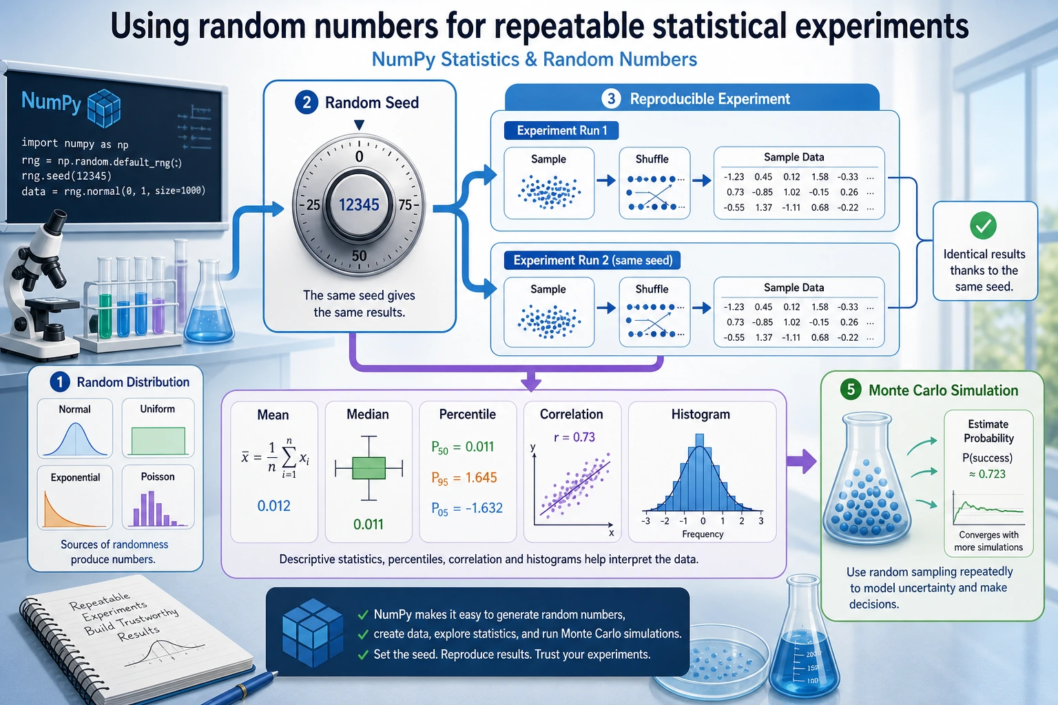
Random Seed: Making “Random” Reproducible

In scientific research and debugging, we often need “reproducible randomness” — getting the same results every time we run the code.

# No seed: different results every time
print(np.random.rand(3))  # Different each time

# Set a seed: same results every time
np.random.seed(42)
print(np.random.rand(3))  # [0.374... 0.950... 0.731...]

np.random.seed(42)        # Reset the same seed
print(np.random.rand(3))  # [0.374... 0.950... 0.731...]  Exactly the same!

# Seed setting with the new API
rng = np.random.default_rng(seed=42)
print(rng.random(3))

rng2 = np.random.default_rng(seed=42)  # Same seed
print(rng2.random(3))                    # Same result

What a Seed Does

A random seed is like a “recipe for random numbers” — the same seed always produces the same sequence of random numbers. Be sure to set a seed in the following situations:

• During learning/tutorials: to make results easier to verify
• In scientific experiments: to ensure results are reproducible
• When debugging code: to remove interference from randomness
• When training machine learning models: to ensure fair comparison experiments

---

Evidence to Keep

Keep this page’s proof of learning as a small evidence card:

Array State

shape, dtype, axis, and sample values before the operation

Operation

indexing, slicing, broadcasting, reshape, linear algebra, or random/stat function

Output

resulting array shape, values, or statistic

Failure Check

axis confusion, view/copy trap, broadcast mismatch, or wrong shape

Expected Output

printed shapes and values that make the array operation inspectable

Common Probability Distributions

Uniform Distribution

Each value has the same probability of appearing:

rng = np.random.default_rng(42)

# Uniform distribution between [0, 1)
uniform_01 = rng.random(10000)
print(f"Mean: {uniform_01.mean():.4f}")  # ≈ 0.5
print(f"Min: {uniform_01.min():.4f}")   # ≈ 0
print(f"Max: {uniform_01.max():.4f}")   # ≈ 1

# Uniform distribution between [low, high)
uniform_custom = rng.uniform(low=10, high=50, size=1000)
print(f"Mean: {uniform_custom.mean():.1f}")  # ≈ 30

Normal Distribution (Gaussian Distribution)

This is one of the most important distributions — it appears everywhere in nature and data:

rng = np.random.default_rng(42)

# Standard normal distribution: mean = 0, standard deviation = 1
standard = rng.standard_normal(10000)
print(f"Mean: {standard.mean():.4f}")  # ≈ 0
print(f"Standard deviation: {standard.std():.4f}")  # ≈ 1

# Normal distribution with a specified mean and standard deviation
# For example: the height of adult men in China is about 170 cm, with a standard deviation of about 6 cm
heights = rng.normal(loc=170, scale=6, size=10000)
print(f"Average height: {heights.mean():.1f} cm")
print(f"Standard deviation: {heights.std():.1f} cm")
print(f"Shortest: {heights.min():.1f} cm")
print(f"Tallest: {heights.max():.1f} cm")

Binomial Distribution

The number of successes in n independent trials (for example, flipping a coin):

rng = np.random.default_rng(42)

# Simulate flipping a coin 10 times (probability of heads = 0.5), repeated 10000 times
results = rng.binomial(n=10, p=0.5, size=10000)
print(f"Average number of heads: {results.mean():.2f}")  # ≈ 5
print(f"Minimum: {results.min()}")
print(f"Maximum: {results.max()}")

Other Common Distributions

rng = np.random.default_rng(42)

# Poisson distribution (number of events)
# For example: 5 customers arrive per hour on average
visitors = rng.poisson(lam=5, size=1000)
print(f"Poisson distribution - Mean: {visitors.mean():.2f}")

# Exponential distribution (time between events)
wait_times = rng.exponential(scale=2.0, size=1000)
print(f"Exponential distribution - Mean: {wait_times.mean():.2f}")

# choice: randomly select from an array
names = np.array(["Alice", "Bob", "Charlie", "Diana", "Eve"])
chosen = rng.choice(names, size=3, replace=False)  # Sampling without replacement
print(f"Random selection: {chosen}")

---

Random Operations

Random Shuffling

rng = np.random.default_rng(42)

arr = np.arange(10)    # [0 1 2 3 4 5 6 7 8 9]

# Shuffle in place
rng.shuffle(arr)
print(arr)              # [8 1 5 0 7 2 9 4 3 6] (random order)

# Shuffle and return a new array (do not modify the original)
arr2 = np.arange(10)
shuffled = rng.permutation(arr2)
print(arr2)       # [0 1 2 3 4 5 6 7 8 9]  original array unchanged
print(shuffled)   # New shuffled array

Random Sampling

rng = np.random.default_rng(42)

data = np.arange(100)

# Sampling with replacement (duplicates possible)
sample1 = rng.choice(data, size=10, replace=True)
print(f"With replacement: {sample1}")

# Sampling without replacement (no duplicates)
sample2 = rng.choice(data, size=10, replace=False)
print(f"Without replacement: {sample2}")

# Weighted random sampling
items = np.array(["Common", "Uncommon", "Rare", "Legendary"])
weights = np.array([0.6, 0.25, 0.1, 0.05])  # probabilities
drops = rng.choice(items, size=20, p=weights)
unique, counts = np.unique(drops, return_counts=True)
for item, count in zip(unique, counts):
    print(f"  {item}: {count} times")

---

Statistical Operations

NumPy provides a rich set of statistical functions:

Descriptive Statistics

rng = np.random.default_rng(seed=42)
data = rng.normal(loc=75, scale=10, size=100)  # Scores of 100 students

print("=== Descriptive Statistics ===")
print(f"Mean (mean):     {np.mean(data):.2f}")
print(f"Median (median): {np.median(data):.2f}")
print(f"Standard deviation (std):    {np.std(data):.2f}")
print(f"Variance (var):      {np.var(data):.2f}")
print(f"Minimum (min):    {np.min(data):.2f}")
print(f"Maximum (max):    {np.max(data):.2f}")
print(f"Range (ptp):      {np.ptp(data):.2f}")   # max - min

Percentiles

rng = np.random.default_rng(seed=42)
data = rng.normal(loc=75, scale=10, size=1000)

# Percentiles
print(f"25th percentile: {np.percentile(data, 25):.2f}")
print(f"50th percentile: {np.percentile(data, 50):.2f}")  # = median
print(f"75th percentile: {np.percentile(data, 75):.2f}")
print(f"90th percentile: {np.percentile(data, 90):.2f}")

# Interquartile range (IQR)
q1 = np.percentile(data, 25)
q3 = np.percentile(data, 75)
iqr = q3 - q1
print(f"Interquartile range (IQR): {iqr:.2f}")

Correlation Coefficient

rng = np.random.default_rng(seed=42)

# Height and weight are usually positively correlated
height = rng.normal(170, 8, 100)
weight = height * 0.6 - 30 + rng.normal(0, 5, 100)  # Approximate linear relationship + noise

# Compute the correlation coefficient matrix
corr_matrix = np.corrcoef(height, weight)
print(f"Correlation coefficient: {corr_matrix[0, 1]:.4f}")  # ≈ 0.7~0.9 (positive correlation)

# Interpretation:
# 1.0  = perfect positive correlation
# 0.0  = no correlation
# -1.0 = perfect negative correlation

Histogram Statistics

rng = np.random.default_rng(seed=42)
scores = rng.normal(75, 10, 200)

# Count how many scores fall into each range
bins = [0, 60, 70, 80, 90, 100]
counts, bin_edges = np.histogram(scores, bins=bins)
labels = ["Failing", "Passing", "Average", "Good", "Excellent"]

print("=== Score Distribution ===")
for label, count, left, right in zip(labels, counts, bin_edges[:-1], bin_edges[1:]):
    bar = "█" * count
    print(f"  {label} [{left:.0f}-{right:.0f}): {count:3d} {bar}")

---

Hands-On: Simulating Monte Carlo

The Monte Carlo method is a classic way to use random numbers to estimate complex problems. Below, we use it to estimate π:

import numpy as np

def estimate_pi(n_points):
    """
    Estimate π by randomly scattering points inside a square
    The proportion of points that fall inside the quarter circle is approximately π/4
    """
    rng = np.random.default_rng(42)

    # Randomly scatter points in the square [0, 1] × [0, 1]
    x = rng.random(n_points)
    y = rng.random(n_points)

    # Compute the distance to the origin
    distance = np.sqrt(x**2 + y**2)

    # Number of points inside the quarter circle (distance <= 1)
    inside = np.sum(distance <= 1)

    # π ≈ 4 × (number of points inside the circle / total number of points)
    pi_estimate = 4 * inside / n_points
    return pi_estimate

# Estimation accuracy with different numbers of points
for n in [100, 1000, 10000, 100000, 1000000]:
    pi_est = estimate_pi(n)
    error = abs(pi_est - np.pi)
    print(f"  {n:>10,} points → π ≈ {pi_est:.6f}  Error: {error:.6f}")

Output summary:

Points	Estimated π	Error
100	3.120000	0.021593
1,000	3.156000	0.014407
10,000	3.153200	0.011607
100,000	3.140480	0.001113
1,000,000	3.142484	0.000891

The more points you use, the more accurate the estimate becomes! That is the charm of the Monte Carlo method.

---

Summary

  root((Random Numbers and Statistics))
    Random Number Generation
      random / rand Uniform distribution
      normal / randn Normal distribution
      integers / randint Random integers
      choice Random selection
      shuffle / permutation Shuffle
    Random Seed
      seed Ensures reproducibility
      default_rng New API
    Probability Distributions
      Uniform distribution uniform
      Normal distribution normal
      Binomial distribution binomial
      Poisson distribution poisson
    Statistical Functions
      mean / median / std / var
      min / max / argmin / argmax
      percentile Percentile
      corrcoef Correlation coefficient
      histogram Histogram

---

Hands-On Exercises

Exercise 1: Simulate Rolling Dice

rng = np.random.default_rng(42)

# Simulate rolling 2 dice 10000 times
# 1. Generate a 10000×2 array of random integers (each row is one roll of two dice)
# 2. Compute the sum of the two dice for each roll
# 3. Count how many times each sum (2~12) appears
# 4. Find the most frequent sum (should be 7)

Exercise 2: Simulate Stock Prices

rng = np.random.default_rng(42)

# Simulate price changes for one stock over 250 trading days
# Initial price: 100
# Daily returns follow a normal distribution: mean 0.05%, standard deviation 2%
initial_price = 100
n_days = 250

# 1. Generate 250 daily returns
# daily_returns = rng.normal(loc=?, scale=?, size=?)

# 2. Compute the price for each day (hint: use np.cumprod)
# prices = initial_price * np.cumprod(1 + daily_returns)

# 3. Compute the final price, highest price, and lowest price
# 4. Compute the annualized return

Exercise 3: Batch Metrics Analysis

rng = np.random.default_rng(seed=42)

# Generate metrics for 200 inference batches
accuracy = rng.normal(0.78, 0.08, 200).clip(0, 1)
latency_ms = rng.normal(180, 35, 200).clip(40, None)

# 1. Compute the mean, standard deviation, and median for each metric
# 2. Compute the correlation coefficient between accuracy and latency
# 3. Count how many batches have accuracy < 0.7 but latency < 160 ms
# 4. Use histograms to analyze both distributions
# 5. Compute the average latency of the top 10 batches by accuracy

---

Reference implementation and walkthrough

• For dice simulation, create a (10000, 2) array, sum along axis=1, and count sums with np.bincount. The most frequent sum should usually be 7 because it has the most combinations.
• For stock simulation, generate daily returns, then compute prices with 100 * np.cumprod(1 + returns). Report the final return, maximum drawdown if asked, and a chart so the path is visible.
• For batch metrics, use mean, std, corrcoef, boolean filters, histograms, and top-k sorting. Always describe the random seed so someone else can reproduce the same sample.

Chapter Summary: A Complete View of NumPy Knowledge

Congratulations on finishing all the NumPy content! Let’s review what you learned in this chapter:

flowchart TB
    subgraph "Chapter 1 NumPy Scientific Computing"
        A["1.1 Overview<br/>Why use NumPy"] --> B["1.2 Array Basics<br/>Creation + Attributes + dtype"]
        B --> C["1.3 Indexing and Slicing<br/>Basic / Boolean / Fancy Indexing"]
        C --> D["1.4 Array Operations<br/>Vectorization + Broadcasting + Aggregation"]
        D --> E["1.5 Reshaping Operations<br/>reshape + Concatenation + Splitting"]
        E --> F["1.6 Linear Algebra<br/>Matrix Multiplication + Inverse + Eigenvalues"]
        F --> G["1.7 Random Numbers and Statistics<br/>Distributions + Sampling + Statistics"]
    end

    G --> H["✅ You now master the core of NumPy!<br/>Ready to move on to Pandas →"]

    style H fill:#4caf50,color:#fff

✅ Self-check: Can you use NumPy to create a 100×3 random matrix, compute the mean and standard deviation of each column, and find the column index of the maximum value in each row?

import numpy as np

rng = np.random.default_rng(42)
matrix = rng.normal(loc=50, scale=15, size=(100, 3))

# Column means
print("Column means:", np.mean(matrix, axis=0))

# Column standard deviations
print("Column standard deviations:", np.std(matrix, axis=0))

# Column index of the maximum value in each row
print("Column indices of row maxima:", np.argmax(matrix, axis=1))

If all of this feels easy — congratulations, you are ready to step into the world of Pandas!