
11.3.3 Deep Learning Text Classification
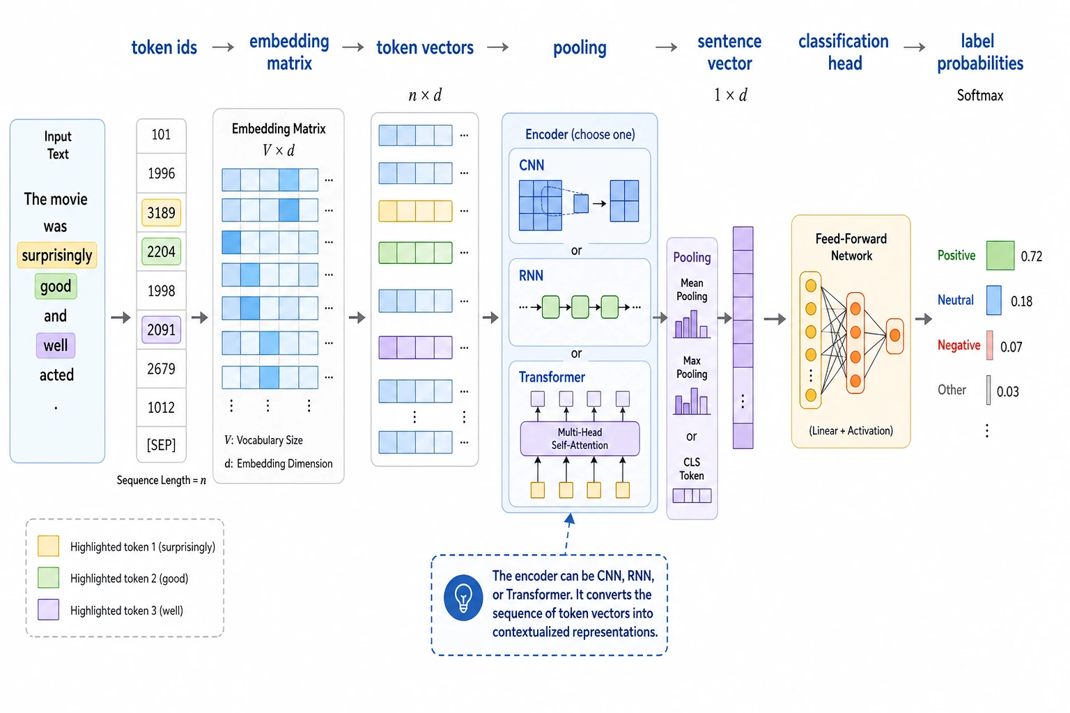
Learning Objectives
Section titled “Learning Objectives”- Understand the core difference between deep learning text classification and traditional methods
- Understand the minimal deep classification pipeline of embedding, pooling, and the classification head
- Build an initial intuition for a “neural text classifier” through a runnable example
- Understand why representation learning changes the upper bound of classification performance
First, build a map
Section titled “First, build a map”Deep learning text classification is easier to understand if you think in terms of “how the input flows”:
flowchart LR A["token"] --> B["embedding"] B --> C["pooling / encoding"] C --> D["sentence representation"] D --> E["classification head"]So the real questions this section wants to answer are:
- What extra capability does a neural text classifier have compared with traditional methods?
- Why does “learn the representation first, then classify” change the performance ceiling?
What does deep learning text classification add beyond traditional methods?
Section titled “What does deep learning text classification add beyond traditional methods?”It no longer relies entirely on hand-crafted features
Section titled “It no longer relies entirely on hand-crafted features”Traditional methods are more like:
- define text features by hand first
- then train a classifier
Deep methods are more like:
- learn the representation and the classification at the same time
The most basic pipeline is actually not complicated
Section titled “The most basic pipeline is actually not complicated”The smallest deep text classifier can usually be broken into:
- token -> embedding
- aggregate a sequence of token representations
- connect a linear classification head
An analogy
Section titled “An analogy”Traditional methods are like first turning a sentence into a table of keywords, then making a judgment. Deep methods are more like first encoding the sentence into a continuous semantic representation, then making a judgment.
A more beginner-friendly overall analogy
Section titled “A more beginner-friendly overall analogy”You can also think of the two methods like this:
- Traditional methods are like checking boxes on a form
- Deep methods are like first getting the gist of a sentence, then drawing a conclusion
The former depends more on:
- which features you decide to inspect in advance
The latter emphasizes more:
- whether the model can learn which expressions are similar to each other on its own
What does the most common minimal neural text classifier look like?
Section titled “What does the most common minimal neural text classifier look like?”Embedding layer
Section titled “Embedding layer”Convert token ids into vectors.
Pooling
Section titled “Pooling”Combine a sequence of token representations into one sentence representation. The simplest one is:
- average pooling
Classification head
Section titled “Classification head”Use a linear layer to map the sentence representation to class scores.
Even though this structure is simple, it already uses continuous representations better than a pure bag-of-words model.
Run a pure Python forward-pass example of a neural text classifier
Section titled “Run a pure Python forward-pass example of a neural text classifier”This code does not train any parameters, but it fully demonstrates:
- token id -> embedding
- pooling
- linear scoring
This way, you can truly understand the minimal skeleton of a “neural text classifier.”
vocab = {    "refund": 0,    "invoice": 1,    "password": 2,    "apply": 3,    "issue": 4,    "reset": 5,}
embedding_table = {    0: [0.9, 0.8, 0.1],    1: [0.2, 0.9, 0.1],    2: [0.1, 0.2, 0.95],    3: [0.8, 0.7, 0.2],    4: [0.2, 0.85, 0.15],    5: [0.1, 0.25, 0.9],}
classifier_weights = {    "refund": [1.0, 0.6, 0.1],    "invoice": [0.2, 1.0, 0.1],    "password": [0.1, 0.1, 1.0],}

def encode(tokens):    return [vocab[token] for token in tokens if token in vocab]

def mean_pool(vectors):    dim = len(vectors[0])    return [sum(vec[i] for vec in vectors) / len(vectors) for i in range(dim)]

def dot(a, b):    return sum(x * y for x, y in zip(a, b))

tokens = ["refund", "apply"]token_ids = encode(tokens)token_vectors = [embedding_table[token_id] for token_id in token_ids]sentence_vector = mean_pool(token_vectors)
scores = {    label: round(dot(sentence_vector, weight), 4)    for label, weight in classifier_weights.items()}
prediction = max(scores, key=scores.get)
print("token_ids:", token_ids)print("sentence_vector:", [round(x, 4) for x in sentence_vector])print("scores:", scores)print("prediction:", prediction)
Expected output:
token_ids: [0, 3]sentence_vector: [0.85, 0.75, 0.15]scores: {'refund': 1.315, 'invoice': 0.935, 'password': 0.31}prediction: refundRead it step by step: the tokens become IDs, IDs become vectors, vectors are averaged into one sentence vector, and the classifier gives the highest score to refund.
Why is this example more useful than directly using nn.Sequential?
Section titled “Why is this example more useful than directly using nn.Sequential?”Because it separates the three key steps:
- embedding
- pooling
- classification
This helps you understand the structure first, and then move on to more complex framework implementations.
Why is pooling so important?
Section titled “Why is pooling so important?”Because classification usually needs a sentence-level representation. Without pooling, you only have a sequence of token vectors, and it is still hard to connect that directly to a classification head.
Let’s look at another minimal example where “similar expressions are easier to bring closer”
Section titled “Let’s look at another minimal example where “similar expressions are easier to bring closer””sentences = { "refund request": [0.85, 0.75, 0.15], "return handling": [0.82, 0.72, 0.18], "password reset": [0.12, 0.15, 0.92],}
def l1_distance(a, b): return round(sum(abs(x - y) for x, y in zip(a, b)), 4)
print("refund request vs return handling:", l1_distance(sentences["refund request"], sentences["return handling"]))print("refund request vs password reset:", l1_distance(sentences["refund request"], sentences["password reset"]))Expected output:
refund request vs return handling: 0.09refund request vs password reset: 2.1The lower distance shows that refund request and return handling are closer in this toy representation. That is exactly the kind of geometry a neural classifier tries to learn from data.
This example is very suitable for beginners because it helps you feel more intuitively that:
- if sentence representations are learned well
- similar expressions should be easier to bring closer together
Why can deep methods often outperform traditional methods?
Section titled “Why can deep methods often outperform traditional methods?”They can use continuous semantic relationships
Section titled “They can use continuous semantic relationships”If “refund request” and “refund processing” have different surface forms but similar meanings, embedding is more likely to pull them closer together.
They can handle context more naturally
Section titled “They can handle context more naturally”Even simple models are already closer to a “representation learning” approach than pure bag-of-words methods.
They can also be extended with stronger structures
Section titled “They can also be extended with stronger structures”Later, you can keep building on top of this with:
- CNN
- RNN
- Transformer
That is the difference in extensibility between deep classification and traditional classification.
When is deep text classification especially worth using?
Section titled “When is deep text classification especially worth using?”There are many ways to express the same thing
Section titled “There are many ways to express the same thing”When the same intent can be phrased in many different ways, deep methods often have an advantage.
Semantics matter more than explicit keywords
Section titled “Semantics matter more than explicit keywords”If keywords alone are not enough to separate classes, deep representations are usually worth trying.
You are willing to accept higher training cost
Section titled “You are willing to accept higher training cost”Compared with traditional methods, deep methods usually mean:
- more training resources
- more complex debugging
The most stable default order when building your first text classification project
Section titled “The most stable default order when building your first text classification project”A more stable order is usually:
- Start with a traditional baseline
- Then use the minimal embedding + pooling model
- Check whether the mistakes are already becoming more stable
- Finally consider stronger architectures or pretrained models
This makes it much easier to see where the gains are coming from than starting with a very complex network right away.
Evidence to Keep
Section titled “Evidence to Keep”Keep this page’s proof of learning as a small evidence card:
- Label Schema
- label definitions and boundary examples
- Dataset Split
- fixed train/test examples or evaluation set
- Prediction
- predicted label, expected label, and confidence or score
- Failure Check
- class imbalance, label overlap, leakage, or confusing wording
- Expected Output
- metrics plus error samples grouped by failure reason
Common misconceptions
Section titled “Common misconceptions”Misconception 1: Deep methods are always better than traditional methods
Section titled “Misconception 1: Deep methods are always better than traditional methods”Not necessarily. For small data, short texts, or tasks with strong rules, traditional methods may already work very well.
Misconception 2: Having embedding automatically means understanding context
Section titled “Misconception 2: Having embedding automatically means understanding context”The minimal embedding + pooling structure is already stronger than bag-of-words, but it is not the same as the strongest form of contextual understanding.
Misconception 3: Only look at the model structure, not the data
Section titled “Misconception 3: Only look at the model structure, not the data”Data quality and label definitions are still extremely important.
If you turn this into a project, what is most worth showing?
Section titled “If you turn this into a project, what is most worth showing?”What is usually most worth showing is not:
- just saying “we used a deep learning model”
but rather:
- the comparison between the traditional baseline and the deep baseline
- how text becomes sentence vectors
- which kinds of expressions are easier to classify correctly with the deep model
- what problems still remain in the failure cases
That makes it easier for others to see:
- that you understand why representation learning is useful
- not just that you changed the model name
Summary
Section titled “Summary”The most important takeaway from this section is to understand deep learning text classification as:
First learn a continuous representation of text, then classify on top of it. Therefore, it is better than traditional bag-of-words methods for tasks with similar semantics, diverse expressions, and more complex context.
Once this intuition is established, learning BERT classification and larger pretrained models later will feel much smoother.
Exercises
Section titled “Exercises”- Change
tokensin the example to["invoice", "issue"]and see how the classification result changes. - Why is pooling a key step in moving from token representations to sentence classification?
- Explain in your own words: what is the core capability that deep classification methods add beyond traditional bag-of-words methods?
- Think about it: in what kinds of tasks would you still prefer trying a traditional baseline first instead of jumping straight to a deep model?
Reference implementation and walkthrough
- Changing tokens to
invoiceandissueshould move the representation toward billing or support intent if those vectors are encoded that way. - Pooling is key because token-level vectors must be summarized into one sentence or document vector before classification.
- Deep methods add the ability to learn composition, order, and context-sensitive representations instead of only counting words.
- Try a traditional baseline first when the dataset is small, labels are unstable, latency matters, or you need interpretable error analysis.