5.3.2 Clustering Algorithms

Section Overview

Clustering means grouping similar samples without labels. The result is not the one true answer; it is a hypothesis about structure that must be checked with metrics, plots, and domain meaning.

What You Will Build

This lesson gives you one practical clustering lab:

• choose K for K-Means with inertia and silhouette score;
• inspect K-Means cluster centers;
• compare K-Means with DBSCAN on curved data;
• tune DBSCAN’s eps;
• run hierarchical clustering as an inspection-friendly alternative.

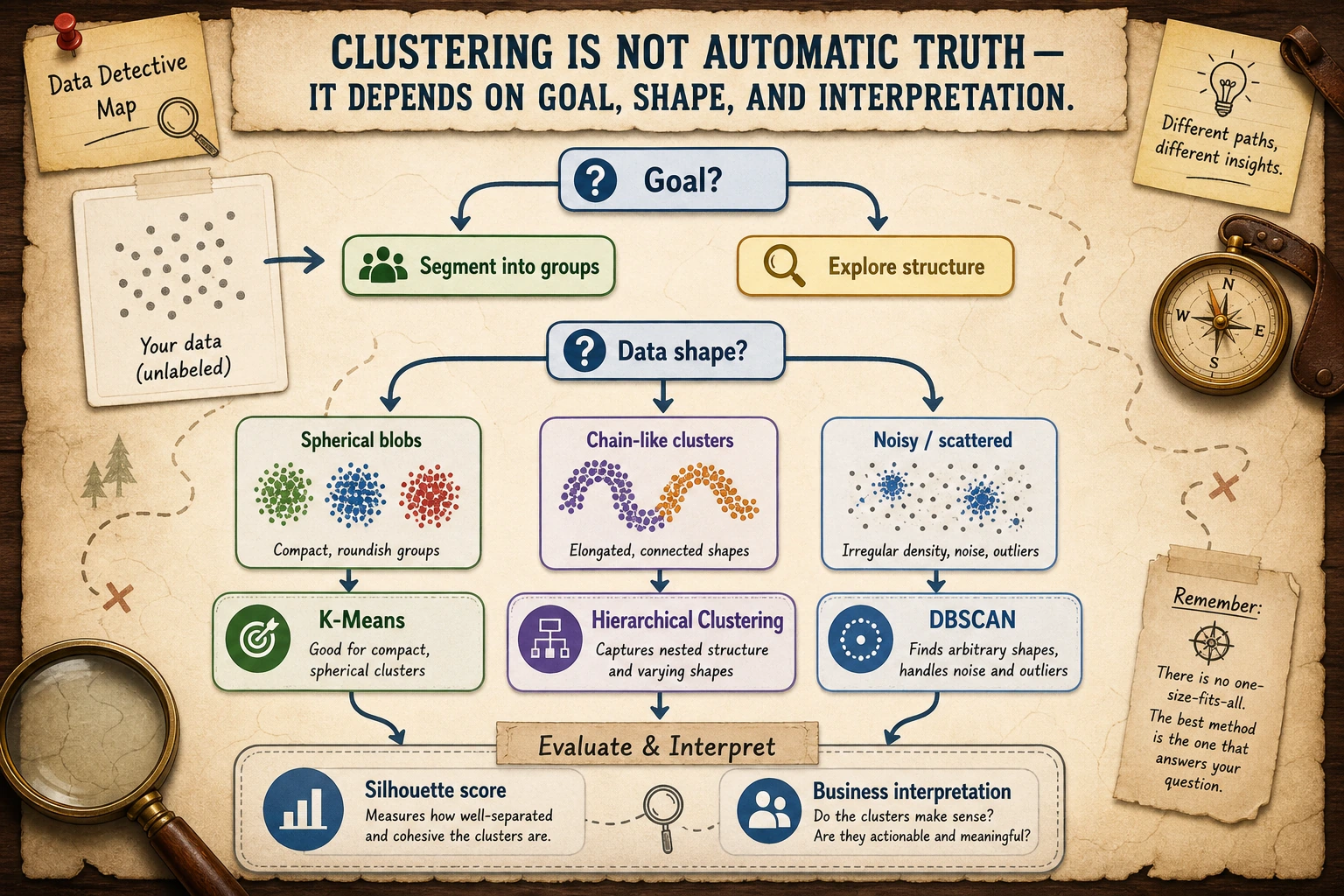
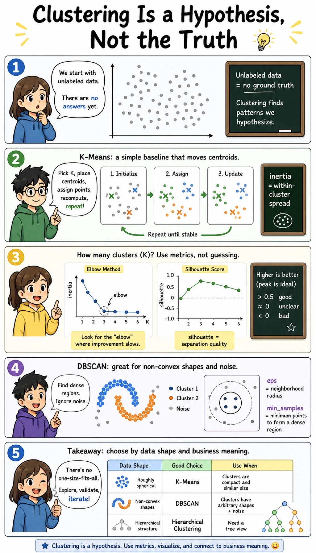
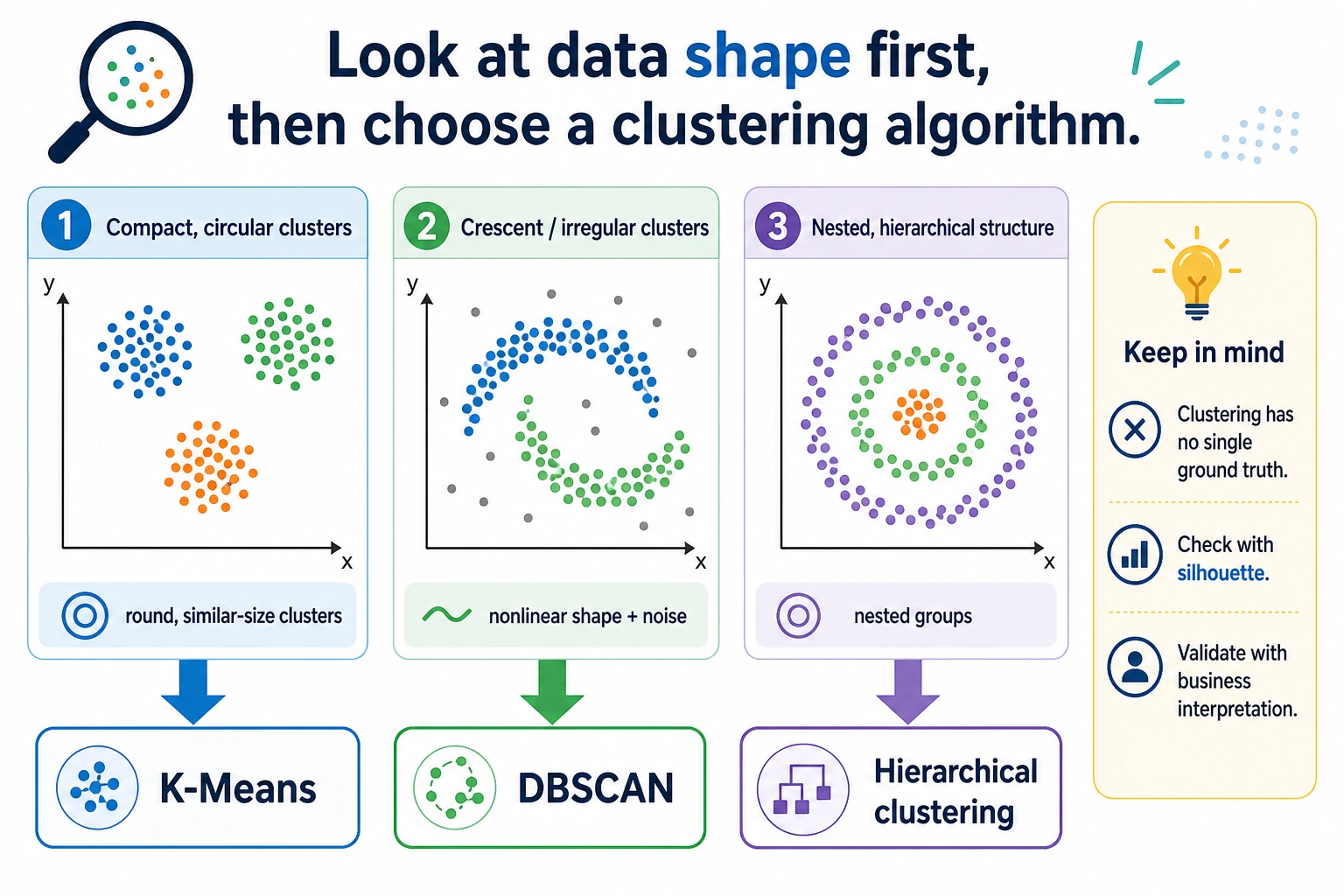
Read the maps first. Clustering is mostly about matching the algorithm’s assumption to the data shape.

Keyword Decoder

Term	Practical meaning
cluster	A group of points that look similar under the chosen features
centroid	The center of a K-Means cluster
inertia_	Within-cluster squared distance; lower is more compact but always drops as K grows
silhouette_score	Measures both compactness and separation; higher is usually better
eps	DBSCAN neighborhood radius
min_samples	Minimum neighbors needed for a dense DBSCAN core point
noise	DBSCAN label -1, meaning “not assigned to a dense cluster”
linkage	Hierarchical clustering rule for merging groups

Setup

python -m pip install -U scikit-learn numpy

All examples scale features first. Clustering is usually distance-based, so feature scale changes the meaning of “similar.”

Run the Complete Lab

Create clustering_lab.py:

import numpy as np
from sklearn.cluster import AgglomerativeClustering, DBSCAN, KMeans
from sklearn.datasets import make_blobs, make_moons
from sklearn.metrics import adjusted_rand_score, silhouette_score
from sklearn.preprocessing import StandardScaler


# Round blob clusters: good K-Means demo.
X_blob, y_blob = make_blobs(n_samples=360, centers=3, cluster_std=0.85, random_state=42)
X_blob = StandardScaler().fit_transform(X_blob)

print("kmeans_k_selection")
for k in [2, 3, 4, 5]:
    model = KMeans(n_clusters=k, n_init="auto", random_state=42)
    labels = model.fit_predict(X_blob)
    print(
        f"k={k} inertia={model.inertia_:6.1f} "
        f"silhouette={silhouette_score(X_blob, labels):.3f}"
    )

best = KMeans(n_clusters=3, n_init="auto", random_state=42)
labels = best.fit_predict(X_blob)
print("kmeans_centers")
print(np.round(best.cluster_centers_, 2))
print("kmeans_ari=", round(adjusted_rand_score(y_blob, labels), 3))

# Curved clusters: DBSCAN is a better fit than K-Means.
X_moon, y_moon = make_moons(n_samples=400, noise=0.08, random_state=42)
X_moon = StandardScaler().fit_transform(X_moon)

print("shape_mismatch_lab")
kmeans = KMeans(n_clusters=2, n_init="auto", random_state=42)
km_labels = kmeans.fit_predict(X_moon)
print("kmeans_moon_ari=", round(adjusted_rand_score(y_moon, km_labels), 3))

for eps in [0.15, 0.25, 0.35]:
    db = DBSCAN(eps=eps, min_samples=5)
    db_labels = db.fit_predict(X_moon)
    clusters = len(set(db_labels)) - (1 if -1 in db_labels else 0)
    noise = int(np.sum(db_labels == -1))
    print(
        f"dbscan eps={eps:.2f} clusters={clusters} noise={noise} "
        f"ari={adjusted_rand_score(y_moon, db_labels):.3f}"
    )

print("hierarchical_lab")
agg = AgglomerativeClustering(n_clusters=3, linkage="ward")
agg_labels = agg.fit_predict(X_blob)
print("agglomerative_ari=", round(adjusted_rand_score(y_blob, agg_labels), 3))

Run it:

python clustering_lab.py

Expected output:

kmeans_k_selection
k=2 inertia= 417.4 silhouette=0.527
k=3 inertia=  16.4 silhouette=0.869
k=4 inertia=  14.6 silhouette=0.690
k=5 inertia=  11.9 silhouette=0.532
kmeans_centers
[[-0.2   1.17]
 [-1.09 -1.25]
 [ 1.29  0.08]]
kmeans_ari= 1.0
shape_mismatch_lab
kmeans_moon_ari= 0.475
dbscan eps=0.15 clusters=12 noise=37 ari=0.312
dbscan eps=0.25 clusters=2 noise=1 ari=0.995
dbscan eps=0.35 clusters=2 noise=1 ari=0.995
hierarchical_lab
agglomerative_ari= 1.0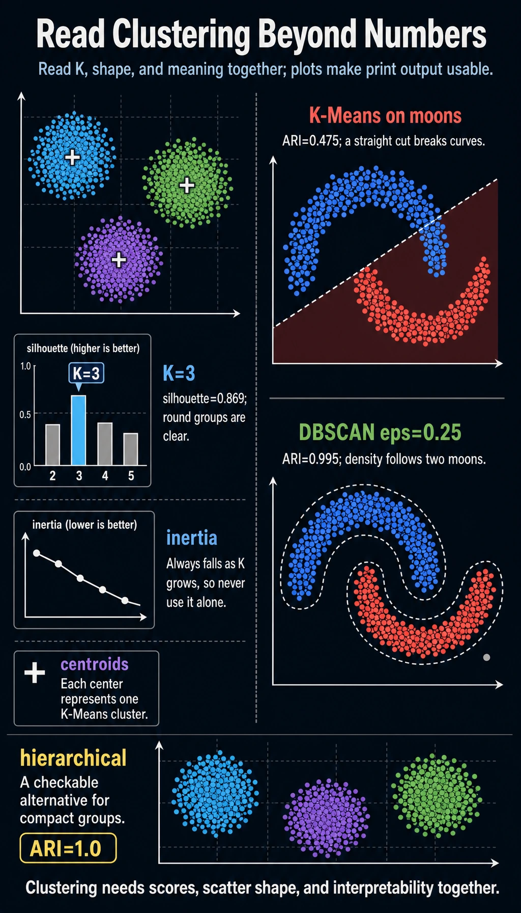

adjusted_rand_score uses the hidden synthetic labels only so this teaching lab can verify behavior. In real clustering work, you usually do not have labels, so you rely on metrics, visualization, and business interpretation.

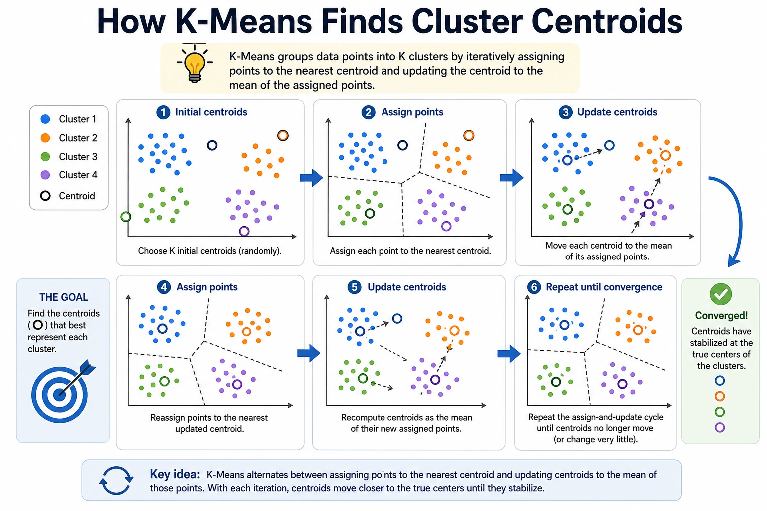
K-Means: Choose K

K-Means repeats three steps:

1. place K centroids;
2. assign each point to the nearest centroid;
3. move each centroid to the mean of its assigned points.

The lab compares candidate K values:

k=2 inertia= 417.4 silhouette=0.527
k=3 inertia=  16.4 silhouette=0.869
k=4 inertia=  14.6 silhouette=0.690

Here K=3 is the best practical choice:

• inertia drops sharply from K=2 to K=3;
• silhouette is highest at K=3;
• adding more clusters lowers inertia but makes the grouping less separated.

Do not choose K from inertia alone. Inertia always improves when K increases, because smaller groups are easier to fit.

K-Means Assumption

K-Means works best when clusters are:

• roughly round;
• similarly sized;
• separated by distance;
• measured on comparable feature scales.

It struggles when clusters are curved, nested, noisy, or very different in density.

DBSCAN: Find Dense Regions

DBSCAN does not ask for K. It asks:

Which points have enough neighbors inside radius eps?

That makes it useful for curved shapes and noisy data. The lab shows the shape mismatch:

kmeans_moon_ari= 0.475
dbscan eps=0.25 clusters=2 noise=1 ari=0.995

K-Means tries to cut the moons into distance-based regions. DBSCAN follows dense curves, so it recovers the two moon shapes.

The key parameter is eps:

dbscan eps=0.15 clusters=12 noise=37
dbscan eps=0.25 clusters=2 noise=1

If eps is too small, DBSCAN breaks one real group into many small pieces. If eps is too large, it can merge groups together.

Hierarchical Clustering

Hierarchical clustering repeatedly merges nearby groups. It is useful when you want to inspect nested relationships or create a dendrogram outside this minimal script.

In the lab:

agglomerative_ari= 1.0

linkage="ward" works well on the round blob data because it prefers compact clusters. For non-round shapes, it may not be enough by itself.

Algorithm Choice

Data shape / goal	Good first choice	Why
Round, compact groups	K-Means	fast, simple, strong baseline
Unknown K, noisy curved shapes	DBSCAN	can mark noise and follow dense regions
Need hierarchy inspection	Agglomerative clustering	shows merge structure
Very high-dimensional embeddings	K-Means or HDBSCAN-style tools	compare with visualization and retrieval checks
Business segmentation	K-Means baseline plus domain review	groups must be actionable, not only pretty

For experienced readers: clustering should be evaluated as a workflow, not just an algorithm score. Check stability under resampling, feature changes, scaling choices, and different random seeds.

Practical Debugging Checklist

Symptom	Likely cause	Fix
K-Means result changes a lot	initialization instability	use n_init="auto", try several seeds
More K always looks better by inertia	inertia always decreases with K	also use silhouette and business interpretability
DBSCAN returns mostly noise	eps too small, features not scaled	scale features, increase eps
DBSCAN returns one giant cluster	eps too large	decrease eps
Clusters look nice but are useless	features do not match actions	define what each cluster will change in the product

Practice

1. Change cluster_std in make_blobs() from 0.85 to 1.5. How does silhouette change?
2. Add K=6 to the K-Means loop. Does inertia improve? Does silhouette improve?
3. Try min_samples=10 in DBSCAN. What happens to noise count?
4. Replace the synthetic data with customer data. Scale numeric features first, then explain each cluster in plain language.
5. Run the same clustering twice with different seeds. Are the groups stable enough to trust?

Reference implementation and walkthrough

1. Increasing cluster_std makes clusters overlap more, so silhouette should usually decrease because points are less clearly closer to their own cluster than to neighboring clusters.
2. Inertia almost always improves when K increases because each point can be closer to some centroid. Silhouette may not improve; if K=6 splits natural groups into fragments, silhouette can drop even while inertia looks better.
3. Larger min_samples makes DBSCAN demand denser neighborhoods. Noise count often increases, and small loose groups may disappear.
4. Customer clusters should be explained with scaled feature averages or medians, not cluster numbers. A useful label might be “high spend, low frequency” rather than “cluster 2.”
5. If different seeds produce very different groups, treat the result as exploration, not a stable segmentation. Compare centroid patterns, silhouette, or adjusted Rand index before trusting the labels.

Evidence to Keep

Keep this page’s proof of learning as a small evidence card:

Task

clustering, dimensionality reduction, or anomaly detection goal

Data View

scaled features, projection, clusters, or anomaly scores

Interpretation

what the groups, axes, or alerts mean in the scenario

Failure Check

arbitrary cluster count, scaling issue, noisy dimension, or false alert

Expected Output

unsupervised result with interpretation and uncertainty note

Pass Check

You are done when you can explain:

• clustering creates a hypothesis, not a guaranteed truth;
• K-Means is a strong baseline for round, compact groups;
• inertia alone cannot choose K;
• DBSCAN is useful for dense curved shapes and noise;
• the final cluster names must be validated by real-world meaning.