6.2.5 nn.Module

Section Overview

nn.Module is how PyTorch packages layers, parameters, forward logic, and training/evaluation mode into one model object. This section upgrades the hand-written parameters from autograd into reusable model classes.

Learning Objectives

• Use nn.Linear and read its parameter shapes.
• Build simple models with nn.Sequential.
• Write a custom nn.Module with __init__() and forward().
• Inspect named_parameters() and state_dict().
• Understand what model.train() and model.eval() actually switch.

---

Look at the Model Container

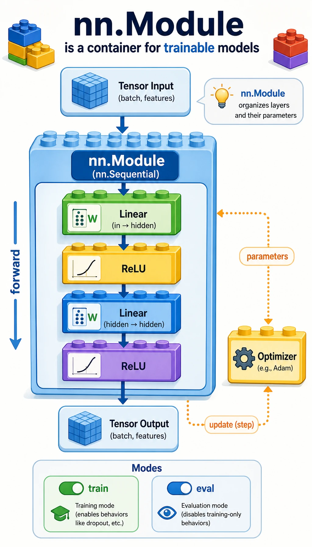
Think of nn.Module as a model container:

layers + parameters + forward logic + mode state -> one model object

The optimizer can then receive model.parameters() without needing to know how many layers you wrote.

From Manual Weights to nn.Linear

In the previous sections, you saw the operation:

logits = X @ W + b

nn.Linear(in_features, out_features) packages the same idea as a trainable layer.

import torch
from torch import nn

layer = nn.Linear(3, 2)

with torch.no_grad():
    layer.weight.copy_(
        torch.tensor(
            [
                [0.1, 0.2, 0.3],
                [-0.1, 0.4, 0.2],
            ]
        )
    )
    layer.bias.copy_(torch.tensor([0.01, -0.02]))

x = torch.tensor([[1.0, 2.0, 3.0]])
y = layer(x)

print("linear_lab")
print("input shape:", tuple(x.shape))
print("weight shape:", tuple(layer.weight.shape))
print("bias shape:", tuple(layer.bias.shape))
print("output:", torch.round(y * 100) / 100)

Expected output:

linear_lab
input shape: (1, 3)
weight shape: (2, 3)
bias shape: (2,)
output: tensor([[1.4100, 1.2800]], grad_fn=<DivBackward0>)

Important shape rule:

• input: [batch, in_features]
• weight: [out_features, in_features]
• output: [batch, out_features]

The printed grad_fn means the output is connected to an autograd graph.

Build a Simple Network with nn.Sequential

Use nn.Sequential when data flows through layers in a straight line.

import torch
from torch import nn

torch.manual_seed(11)

model = nn.Sequential(
    nn.Linear(3, 4),
    nn.ReLU(),
    nn.Linear(4, 2),
)

batch = torch.randn(5, 3)
logits = model(batch)

print("logits shape:", tuple(logits.shape))

Expected output:

logits shape: (5, 2)

Read the model:

[batch, 3]→Linear(3, 4)→ReLU→Linear(4, 2)→[batch, 2]

That is already a small multilayer perceptron.

Write a Custom nn.Module

Custom modules are the normal style for real projects because they can hold named submodules, branching logic, reusable helper methods, and clearer debugging hooks.

import torch
from torch import nn


class TinyClassifier(nn.Module):
    def __init__(self, in_features=3, hidden=4, classes=2):
        super().__init__()
        self.net = nn.Sequential(
            nn.Linear(in_features, hidden),
            nn.ReLU(),
            nn.Linear(hidden, classes),
        )

    def forward(self, x):
        return self.net(x)


torch.manual_seed(11)
model = TinyClassifier()
batch = torch.randn(5, 3)
logits = model(batch)

print("module_lab")
print("logits shape:", tuple(logits.shape))
for name, param in model.named_parameters():
    print(name, tuple(param.shape))
print("state keys:", list(model.state_dict().keys()))

Expected output:

module_lab
logits shape: (5, 2)
net.0.weight (4, 3)
net.0.bias (4,)
net.2.weight (2, 4)
net.2.bias (2,)
state keys: ['net.0.weight', 'net.0.bias', 'net.2.weight', 'net.2.bias']

Responsibilities:

Method or API	Responsibility
__init__()	create layers and submodules
forward()	describe how input becomes output
parameters()	return learnable parameters for the optimizer
named_parameters()	expose parameter names and shapes for debugging
state_dict()	expose tensors that can be saved and loaded

Keep training logic out of forward(). Loss, backward(), and optimizer.step() belong to the training loop, not to the model definition.

How to Read the Model

When you inspect an nn.Module, read it at three levels:

Level	Question	Evidence
structure	what layers exist and in what order?	print(model)
parameters	which tensors will be trained?	named_parameters()
behavior	what does forward() return for one batch?	one input/output shape check

If all three are clear, the model is no longer a black box. It is a Python object with trainable tensors and an explicit forward path.

train() and eval() Are Mode Switches

model.train() does not run the training loop, and model.eval() does not run validation. They switch the behavior of layers such as Dropout and BatchNorm.

Run this example:

import torch
from torch import nn


class DropoutProbe(nn.Module):
    def __init__(self):
        super().__init__()
        self.dropout = nn.Dropout(p=0.5)

    def forward(self, x):
        return self.dropout(x)


probe = DropoutProbe()
sample = torch.ones(6)

torch.manual_seed(3)
probe.train()
train_a = probe(sample)
train_b = probe(sample)

probe.eval()
eval_a = probe(sample)
eval_b = probe(sample)

print("mode_lab")
print("train outputs equal:", torch.equal(train_a, train_b))
print("eval outputs equal:", torch.equal(eval_a, eval_b))
print("eval output:", eval_a)

Expected output:

mode_lab
train outputs equal: False
eval outputs equal: True
eval output: tensor([1., 1., 1., 1., 1., 1.])

Practical habit:

model.train()  # before training batches
model.eval()   # before validation or prediction

For validation, combine it with torch.no_grad():

model.eval()
with torch.no_grad():
    logits = model(batch)

Mini Project: Train a Score Predictor

This example uses two features and one regression target:

• study hours per week;
• practice problems completed per week;
• predicted score.

The target is divided by 100 so the optimization is stable on this tiny dataset.

import torch
from torch import nn


class ScorePredictor(nn.Module):
    def __init__(self):
        super().__init__()
        self.net = nn.Sequential(
            nn.Linear(2, 16),
            nn.ReLU(),
            nn.Linear(16, 1),
        )

    def forward(self, x):
        return self.net(x)


torch.manual_seed(42)

X = torch.tensor(
    [
        [2.0, 1.0],
        [3.0, 2.0],
        [4.0, 3.0],
        [5.0, 5.0],
        [6.0, 6.0],
        [7.0, 8.0],
    ]
)
y = torch.tensor(
    [
        [55.0],
        [60.0],
        [68.0],
        [78.0],
        [85.0],
        [92.0],
    ]
) / 100.0

model = ScorePredictor()
loss_fn = nn.MSELoss()
optimizer = torch.optim.Adam(model.parameters(), lr=0.03)

print("training_lab")
for epoch in range(401):
    pred = model(X)
    loss = loss_fn(pred, y)

    optimizer.zero_grad()
    loss.backward()
    optimizer.step()

    if epoch % 100 == 0:
        print(f"epoch={epoch:3d} loss={loss.item():.4f}")

model.eval()
with torch.no_grad():
    test = torch.tensor([[6.5, 7.0]])
    pred_score = model(test).item() * 100

print("predicted score:", round(pred_score, 2))

Expected output:

training_lab
epoch=  0 loss=0.4672
epoch=100 loss=0.0003
epoch=200 loss=0.0001
epoch=300 loss=0.0001
epoch=400 loss=0.0001
predicted score: 89.31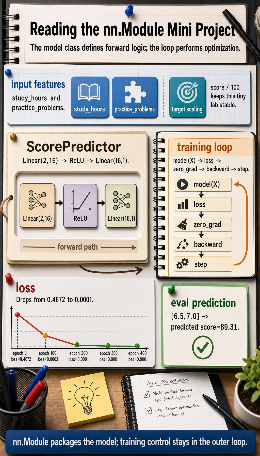

This is now a complete miniature PyTorch model:

data→model→loss→zero_grad→backward→optimizer.step→eval prediction

Evidence to Keep

For this page, save evidence that the model object is understandable, not just runnable:

Structure Check

print(model) or write the layer order

Parameter Check

named_parameters() with shape for each trainable tensor

State Dict Keys

checkpoint keys that would be saved

Mode Probe

train outputs differ, eval outputs match for DropoutProbe

Mini Project Result

loss decreases and predicted score is near the expected range

This proves you can inspect a PyTorch model before trusting a training run. If a later project fails, these same checks tell you whether the problem is model structure, parameter registration, mode switching, or training logic.

Sequential or Custom Module?

Situation	Good choice
simple straight-line stack	nn.Sequential
multiple inputs or outputs	custom nn.Module
skip connections or branches	custom nn.Module
reusable components	custom nn.Module
you need clearer parameter names	custom nn.Module

In real deep learning projects, custom modules are more common because architectures quickly become more than a straight line.

Common Mistakes

Mistake	Why it hurts	Fix
creating layers inside forward()	new parameters are created on every call and may not be optimized correctly	define layers in __init__()
putting loss and optimizer logic inside forward()	mixes model definition with training control	keep forward() as input-to-output only
forgetting super().__init__()	submodules may not register correctly	call it first in __init__()
not checking parameter names	hard to debug frozen or missing layers	print named_parameters()
forgetting eval() for validation	Dropout/BatchNorm behave like training	call model.eval() before validation

Exercises

1. Change the hidden size in ScorePredictor from 16 to 4 and 32. How does the loss change?
2. Remove ReLU(). Does the model still learn this tiny regression task? Why might deeper nonlinear tasks need it?
3. Print model.state_dict() keys and shapes. Which tensors would be saved in a checkpoint?
4. Add nn.Dropout(p=0.2) after ReLU, then compare predictions in train() and eval() modes.

Reference implementation and walkthrough

1. 4 may underfit because the hidden representation is smaller. 32 may reduce training loss more easily, but validation loss is the real check because a larger model can also overfit.
2. This tiny regression task may still learn if the target is close to linear. Without nonlinear activations, stacked linear layers collapse into one linear transformation, which is not enough for richer nonlinear patterns.
3. state_dict() saves learnable tensors such as Linear weights and biases. Layers like Dropout have behavior but no learnable parameter tensor to save.
4. In train() mode, dropout randomly masks activations and predictions can vary between calls. In eval() mode, dropout is disabled, so predictions should be stable.

Key Takeaways

• nn.Module manages layers, parameters, forward logic, and mode state together.
• forward() should describe data flow, not the training loop.
• model.parameters() is what connects the model to the optimizer.
• state_dict() is the standard checkpoint interface.
• train() and eval() switch layer behavior; they do not run loops by themselves.